
What is $ in Excel
 By
SpreadCheaters
By
SpreadCheaters
Excel has a built-in list of special characters that can be used inside the formulas. Each of them represents a special meaning and they perform different functions in Excel formulas and custom functions as well.
The “$” sign is also one of these special characters and it is used in formulas to create an Absolute Reference to the cell. Absolute Reference, when used with a cell’s name, the reference to that specific cell does not change while dragging down the formula along the rows of the column. Let’s explore the following example data set where we wish to calculate the percent discount on the cost of the items. Let’s do this by following the steps explained below;
Step 1 – Convert the percent discount to percentage format
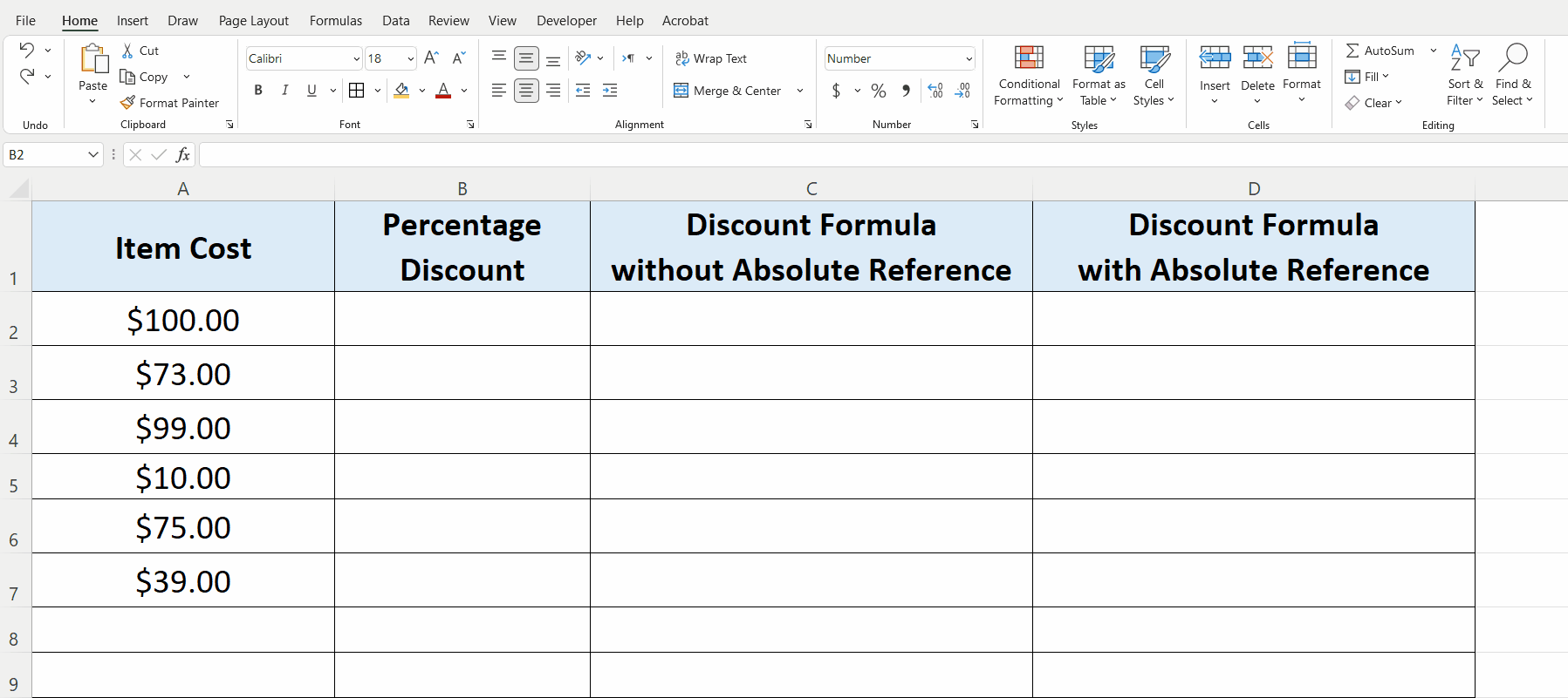
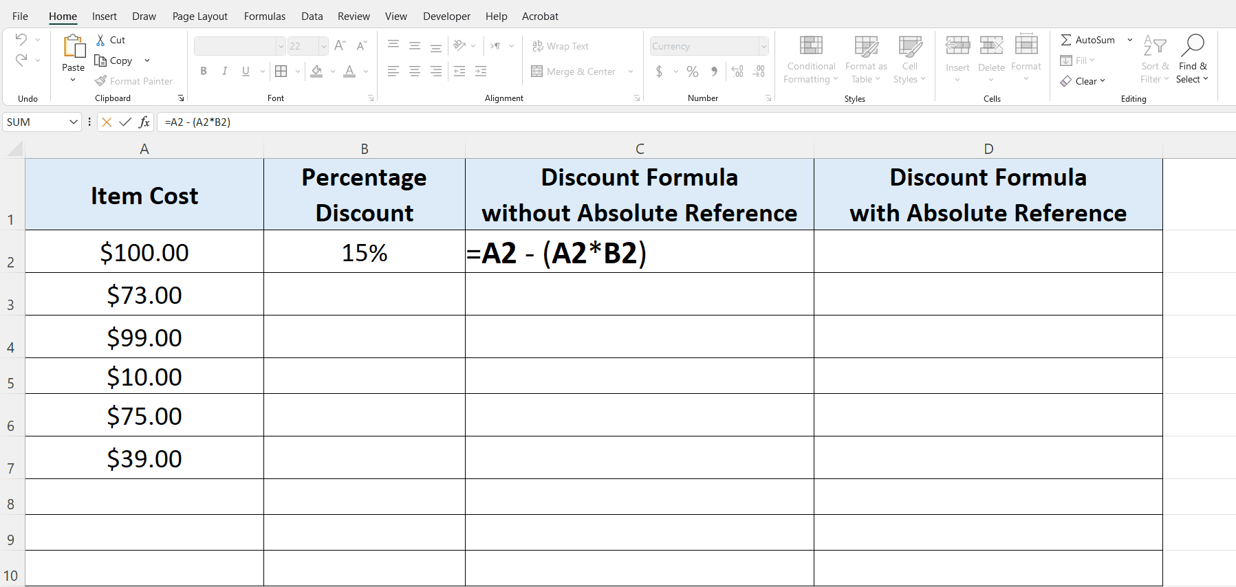
– Let’s suppose we wish to calculate a 15% discount on every item’s cost. For this we’ll enter =15/100 in cell B2. This will give us an answer in decimal point format which is not very friendly. We’ll convert that to percent format by clicking on the % sign in the Number group on the HOME tab as shown below;
Step 2 – Implement the percentage formula without Absolute Reference
– To calculate the percentage discount in column C we will use the generic formula
Cost of item – (Cost of item x percent discount)
In the first case we’ll use the formula without Absolute Reference to show the problems associated with it.
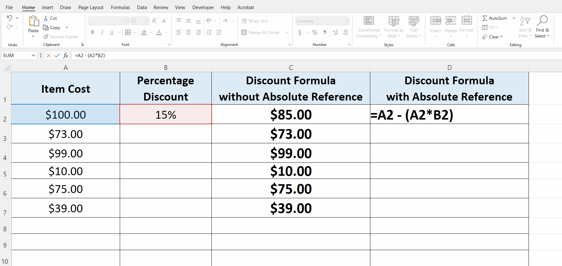
– The actual formula in this case will be as follows. Implement it in the cell C2 and drag down the formula as shown below;
=A2 – (A2 * B2)
As you can see in the picture above, when we dragged down the formula we got incorrect results except the cell C2 where we actually implemented the formula. When we dragged down the formula, the cell reference (B2) to the number used to calculate percentage, was changed also to B3, B4 etc.
Now let’s see how we can rectify this issue by using Absolute Cell Reference.
Step 3 – Implement the percentage formula with Absolute Reference

– Now we will implement the same formula but with slight change in writing B2 in the formula. The new formula will be as follows;
=A2 – (A2 * $B$2)
The new $ sign in “$B$2” means that the reference to cell B2 is fixed or we can say that it is now converted to Absolute Cell Reference.
– To convert a non absolute reference to absolute just move the cursor to the cell name in the formula and press F4. Now the reference to B2 will not change while dragging down the formula along the column as shown in the figure above;
This time we saw that the cell reference to B2 is not changed while dragging down the formula and all percentages were calculated according to the actual value.


