What is cell name box and how to use it in Excel

In this tutorial we’ll learn about the cell name box and how to use it in Excel.

What is a Cell Name Box

Every cell has a specific name according to its column name and row number. It is located at the left corner of Microsoft Excel main worksheet just below the icon bar. It’s just before the formula bar , and the default name of the cell is A1, which is set at start. Microsoft Excel provides a specific box to identify the current selected cell name. This box allows us to type any cell name and it will take us to that location so we do not have to drag and search the exact location of that particular cell. In some cases we have multiple tables in our worksheet. By using the cell name box we can select the tables of our choice. Microsoft Excel will take us to that table , we do not have to search in a big worksheet. 

Let’s see how to use this cell name box in the following steps.

Microsoft Excel is a world’s powerful mathematical calculations tool. It can manipulate data in millions of different ways. Microsoft Excel has a basic storage unit called the cell.

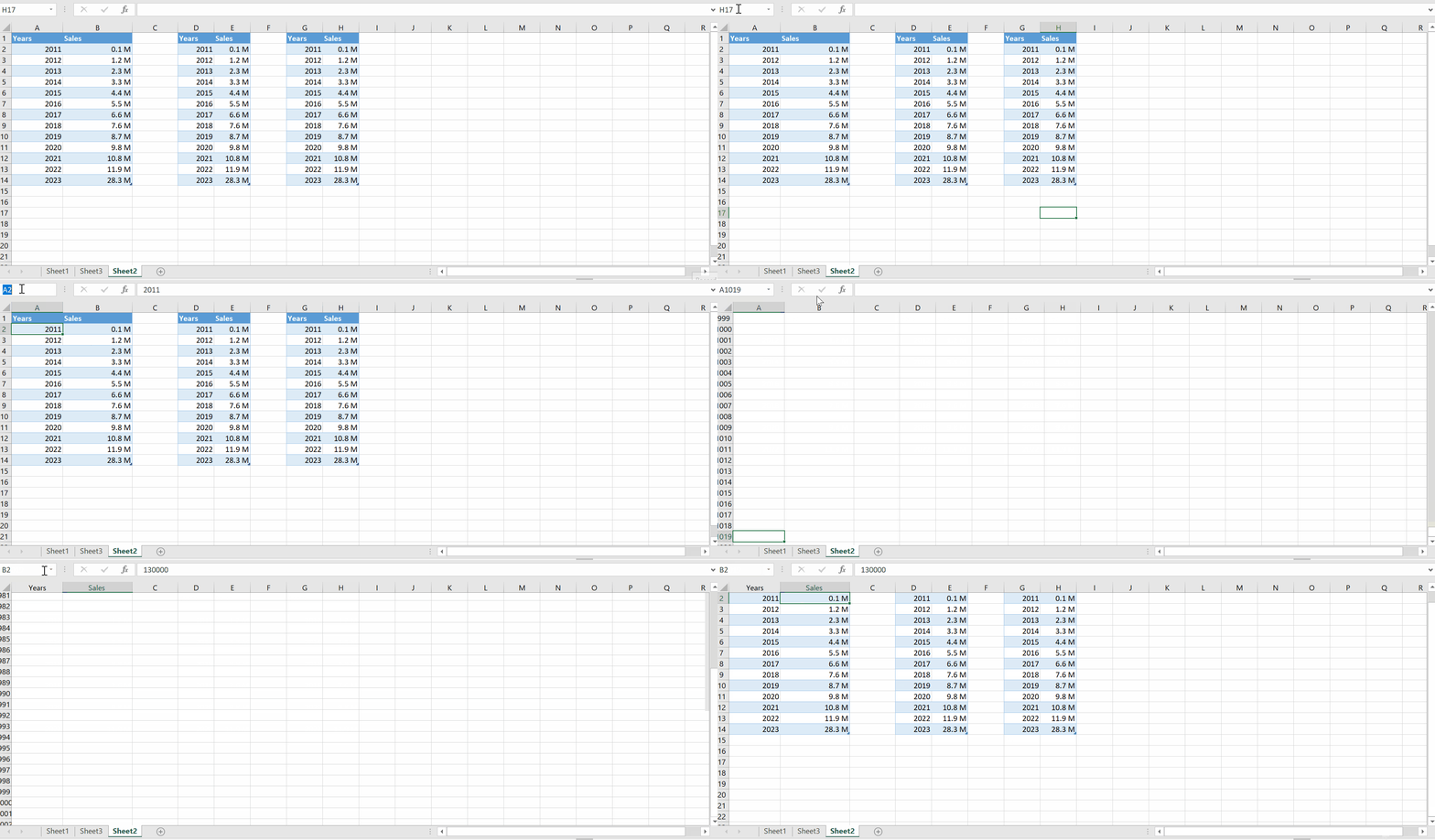
Step 1 – Use the cell name box to jump to any cell in the sheet

Animation is given above;

– Open worksheet.
– Click on the cell name box.
– Type your desired cell number.
– Excel will take you to that location. In this way, you can jump to any particular cell in the sheet without scrolling to that cell.

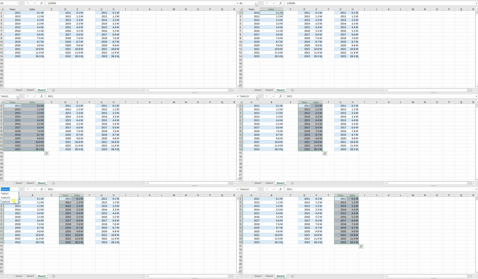
Step 2 – Use name box to select tables

Animation is given above;

– Open worksheet.
– Click on the cell name box.
– If your sheet has various tables then a drop down menu will appear, showing you all the names of the tables present in the sheet.
– Select the table name of your choice.
– Excel will take you to that table. This is particularly helpful when you have a very big sheet with lots of tables in it.