
Using COUNTIFS in Excel to find values greater than a specified criteria
 By
SpreadCheaters
By
SpreadCheaters
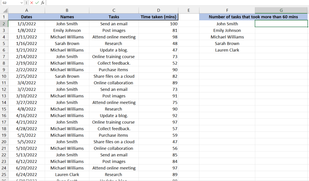
We have a dataset that includes information about people performing online tasks on various dates, along with the time it took them to complete each task in minutes. The dataset includes instances where individuals have completed tasks on multiple dates, and some of those tasks took longer than 60 minutes. We want to determine the number of tasks completed by each person that exceeded 60 minutes.
Follow the simple steps given below to learn how to use COUNTIFS Function:
Understanding the formula
The general syntax of the COUNTIFS function is as follows:
COUNTIFS(range1, criteria1, [range2, criteria2], …)
range1 is the first range of cells that you want to evaluate.
criteria1 is the condition or criteria that you want to apply to range1.
[range2, criteria2] (optional) represents additional ranges and criteria you can specify. You can have multiple pairs of ranges and criteria.
… (ellipsis) indicates that you can continue adding more range-criteria pairs if needed.
COUNTIFS is a function commonly used in spreadsheet programs, such as Microsoft Excel or Google Sheets, to count the number of cells that meet multiple specified criteria. It allows you to apply multiple conditions to a range of cells and counts only the cells that satisfy all the given conditions. We use the COUNTIFS function with the “greater than” criterion (>) when we want to count the number of cells that meet a specific condition of being greater than a certain value.
Step 1 – Selecting the cell
– First of all, select any vacant cell in which you want to use the formula to be implemented and get the results there.
– This is the cell where we will apply the COUNTIF function with greater than criteria.
Step 2 – Writing the formula
– After selecting the cell, press the = button on your keyboard.
– Then, Write COUNTIFS and select the COUNTIFS Function by pressing the tab button on your keyboard. Your formula would look like this,
=COUNTIFS(B2:B41,F2,D2:D41,”>60″
Step 3 – Implementing the formula
– Once you’ve written the formula, add the closing parenthesis.
– Then, press Enter to get the results.
– The result of the formula is 7, indicating that the person mentioned in cell F2 has completed 7 tasks that took more than 60 minutes.
Step 4 – Applying the formula to the whole range
– For applying the formula on the whole range, select the cell in which the result is present. For example, it is a G2 cell in our case.
– Then move your cursor to the right bottom corner of the cell, and your cursor would turn into a + shape which is called the fill handle.
– Double-Click on this fill handle and the formula would be applied to the whole range.


