If the cell contains specific text then return the value

In Excel, the phrase “if the cell contains specific text then return the value” refers to a formula or function that allows you to check if a cell contains a particular text or string, and if it does, it returns a specified value or performs a specific action. The overall importance of this functionality in Excel is significant because it allows you to analyze and manipulate data based on specific conditions. 

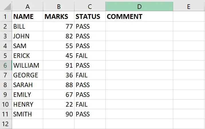
We have a dataset that includes the results of a class, containing the names of students, their corresponding marks, and their pass or fail status. Our goal is to provide comments on each result based on the status. If a student has passed, we want to offer congratulations, and if they have failed, we want to suggest trying again. For this, we have 4 methods. 

Method 1: Return the Value using the IF and the EXACT functions

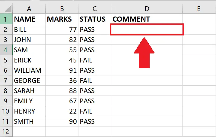
Step 1 – Select the cell

• Select the cell where you want to show the result

Step 2 – Type the Formula

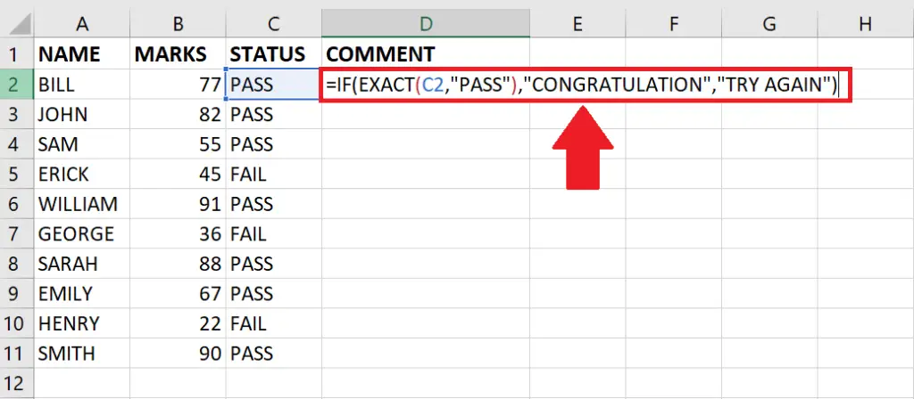
• After selecting the cell, type the following formula
• =IF(EXACT(C2,”PASS”),”CONGRATULATION”,”TRY AGAIN”)
• In this formula, C2 is the cell containing the status (PASS or FAIL). If the status is exactly “PASS,” the formula will return “CONGRATULATIONS”; otherwise, it will return “TRY AGAIN.”

Step 3 – Press the Enter key

• After typing the formula, press the Enter key to get the result

Step 4 – Apply the Formula to the Complete Column

• After getting the result in the cell, drag it to the required cell of the column to apply the formula to the complete column

Method 2:  Return the Value using the IF, ISNUMBER, and SEARCH functions

Step 1 – Select the cell

• Select the cell where you want to show the result

Step 2 – Type the Formula

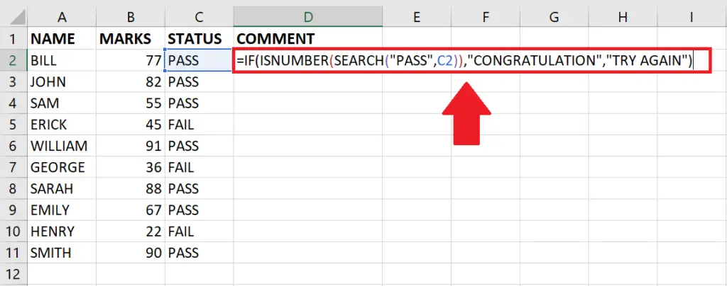
• After selecting the cell, type the following formula
• =IF(ISNUMBER(SEARCH(“PASS”,C2)),”CONGRATULATION”,”TRY AGAIN”)
• In this formula, C2 is the cell containing the status (PASS or FAIL). If the status contains the text “PASS” (case-insensitive), the formula will return “CONGRATULATIONS”; otherwise, it will return “TRY AGAIN.”

Step 3 – Press the Enter key

• After typing the formula, press the Enter key to get the result

Step 4 – Apply the Formula to the Complete Column

• After getting the result in the cell, drag it to the required cell of the column to apply the formula to the complete column

Method 3: Return the Value using the IF and the COUNTIF functions

Step 1 – Select the cell

• Select the cell where you want to show the result

Step 2 – Type the Formula

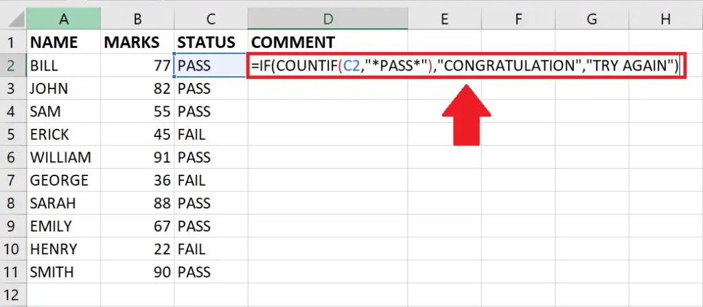
• After selecting the cell, type the following formula
• =IF(COUNTIF(C2,”*PASS*”),”CONGRATULATION”,”TRY AGAIN”)
• In this formula, C2 is the cell containing the status (PASS or FAIL). The COUNTIF function checks if the status contains the text “PASS” anywhere within it. If there is a match (count greater than zero), the formula will return “CONGRATULATIONS”; otherwise, it will return “TRY AGAIN.”

Step 3 – Press the Enter key

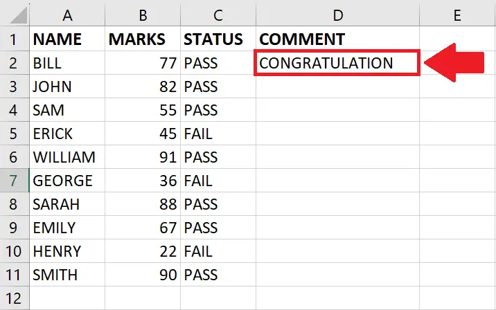
• After typing the formula, press the Enter key to get the result

Step 4 – Apply the Formula to the Complete Column

• After getting the result in the cell, drag it to the required cell of the column to apply the formula to the complete column

Method 4: Return the Value using the IF functions

Step 1 – Select the cell

• Select the cell where you want to show the result

Step 2 – Type the Formula

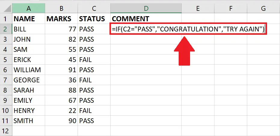
• After selecting the cell, type the following formula
• =IF(C2=”PASS”,”CONGRATULATION”,”TRY AGAIN”)
• In this formula, C2 is the cell containing the status (PASS or FAIL). If the status is exactly equal to “PASS”, the formula will return “CONGRATULATIONS”; otherwise, it will return “TRY AGAIN”.

Step 3 – Press the Enter key

• After typing the formula, press the Enter key to get the result

Step 4 – Apply the Formula to the Complete Column

• After getting the result in the cell, drag it to the required cell of the column to apply the formula to the complete column