How to write ratios in Excel.
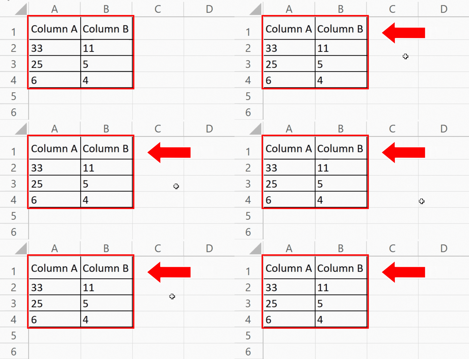
We will use a sample data set with two columns, Column A and Column B, to demonstrate ratio calculations. The values in Column B correspond to the denominator, while those in Column A correspond to the numerator. The ratio of each numerator value to its corresponding denominator value, expressed in the form A: B, is what we want to display in a third column.
Microsoft Excel is a robust spreadsheet program with a number of features for analyzing and manipulating data. The calculation and presentation of ratios is one practical use of Excel. Ratios enable quick comparisons by shedding light on the connections between various data points. This step-by-step documentation will walk you through the process of writing ratios in Excel, giving you the ability to express proportional relationships in an organized, clear manner.
Step 1 – Open the Spreadsheet:
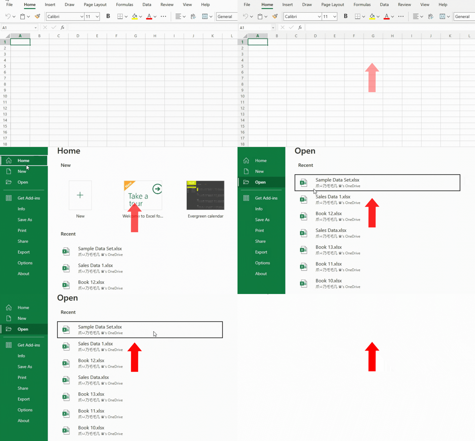
– Open Microsoft Excel.
– Navigate to the spreadsheet containing the data set.
Step 2 – Select the cell where you want to display the output:
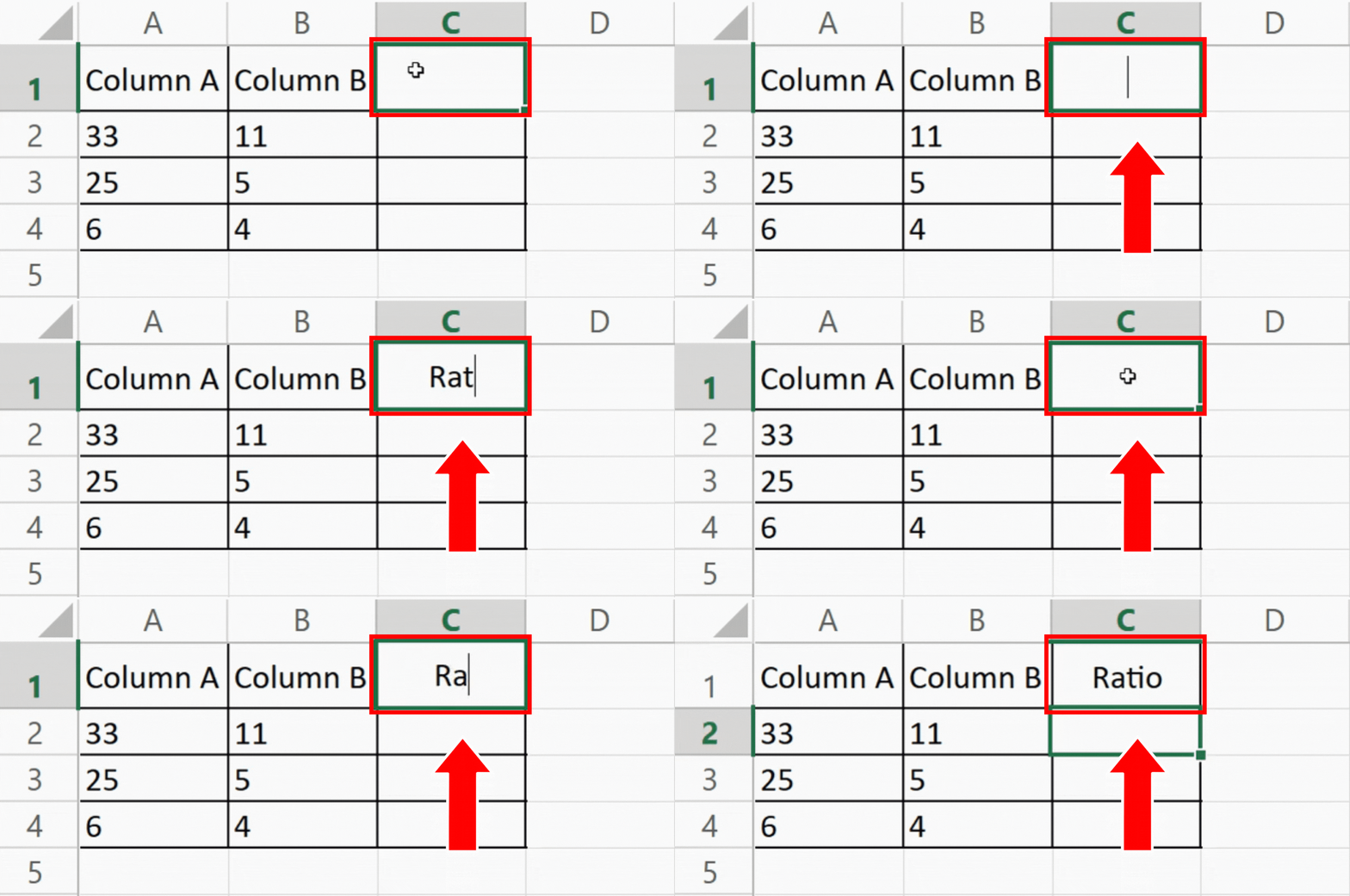
– Choose the cells in which you want to show the ratios.
– In this instance, let’s say Column C, we will create the ratios in a new column.
Step 3 – Enter the formula:
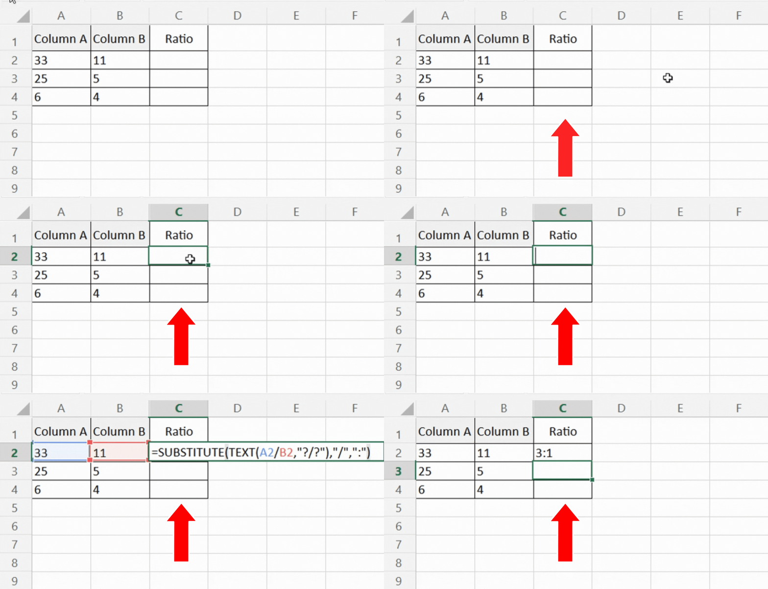
– Enter the following formula in the first cell (C1) of the new column:
=SUBSTITUTE(TEXT(A2/B2,”?/?”),”/”,”:”).
– Here, the outcome of the division of A1/B1 is transformed into an improper fraction using the TEXT function.
– The fraction’s “/” is changed to a colon (“:”) using the SUBSTITUTE function.
– To apply the formula to the first cell, press Enter.
Step 4 – Apply the formula to the remaining cells:

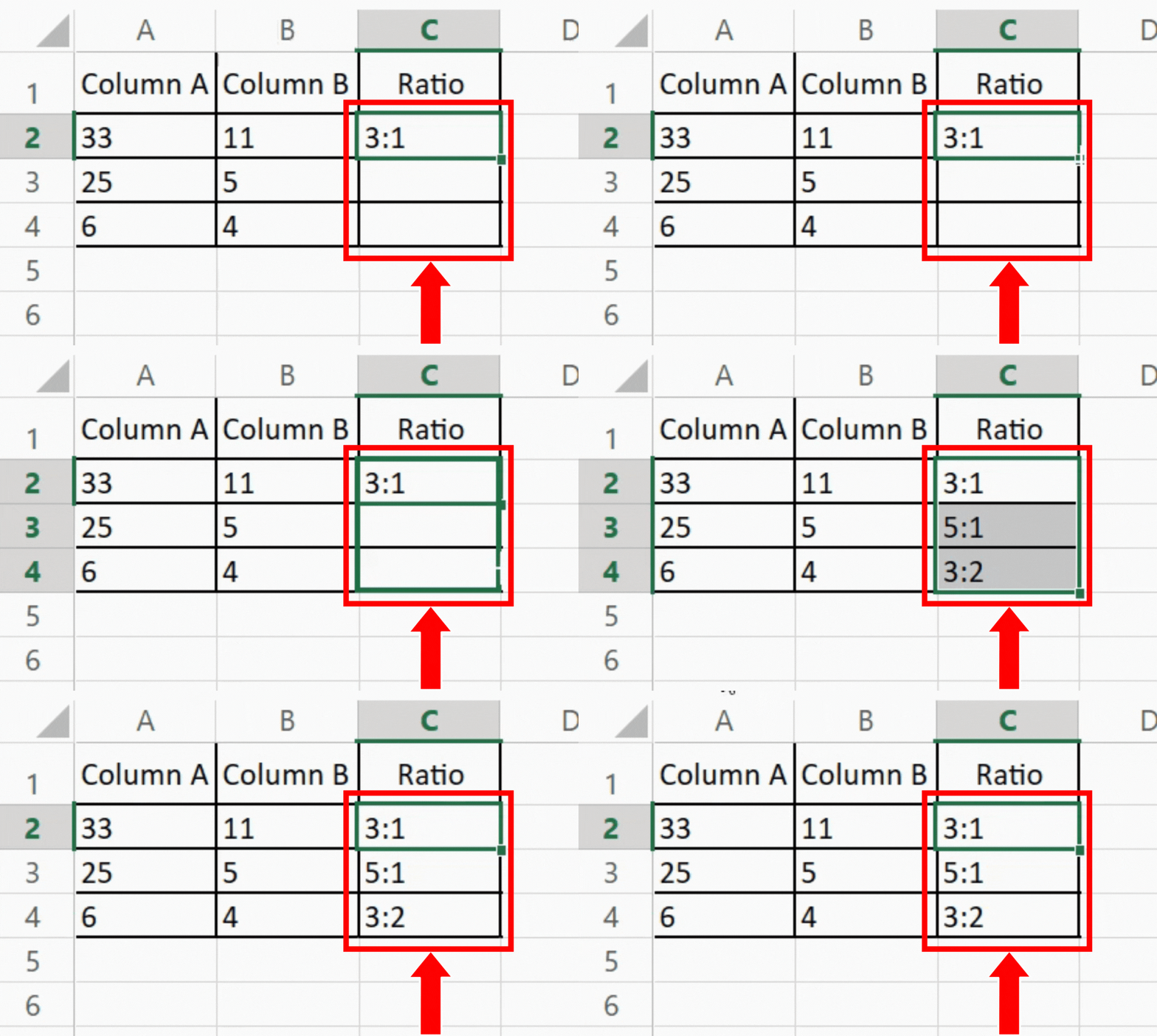
– Now the first row’s ratio is computed. There are two ways to apply the formula to the remaining rows.
– Double-click the small square in the cell marked C1‘s bottom right corner. This will automatically adjust the cell references and copy the formula to the remaining cells in Column C.
– Or you can, select the range of cells in Column C where you want to apply the formula, copy the formula (C1), and then paste the formula into the chosen cells.
Conclusion:
You have successfully written ratios in Excel by following these steps. The ratios of each numerator value to its corresponding denominator value are now shown in the newly created Column C in the desired format of A:B. The convenience of performing calculations and presenting data in different formats made possible by Excel’s built-in functions allows for effective analysis and the visual representation of proportional relationships.


