How to wrap around text In Excel

Microsoft Excel is designed to calculate and manipulate numbers. However, you may often find yourself in situations when, in addition to numbers, large amounts of text need to be stored in spreadsheets. In such cases, longer text does not fit completely in a cell, you can of course proceed with the most obvious way and simply make the column wider. However, it’s not really an option when you work with a large worksheet that has a lot of data to display.

A much better solution is to wrap text that exceeds a column width, and Microsoft Excel provides a couple of ways to do it. This tutorial will introduce you to the Excel wrap text feature.

What is Wrap Text in Excel?

When the data input in a cell is too large to fit in it, one of the following two things happens:

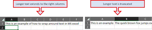
• If columns to the right are empty, a long text string extends over the cell border into those columns.
• If an adjacent cell to the right contains any data, a text string is cut off at the cell border.

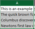
The below screenshot shows two cases:

The wrap text feature can help you fully display longer text in a cell without overflowing it to other cells. “Wrapping text” means displaying the cell contents on multiple lines, rather than one long line. This will allow you to avoid the “truncated column” effect, make the text easier to read and better fit for printing. In addition, it will help you keep the column width consistent throughout the entire worksheet.

Use one of the following methods to force a lengthy text string to appear on multiple lines.

 Method 1 – Wrap Text Button

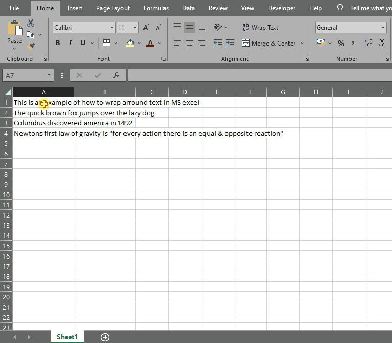
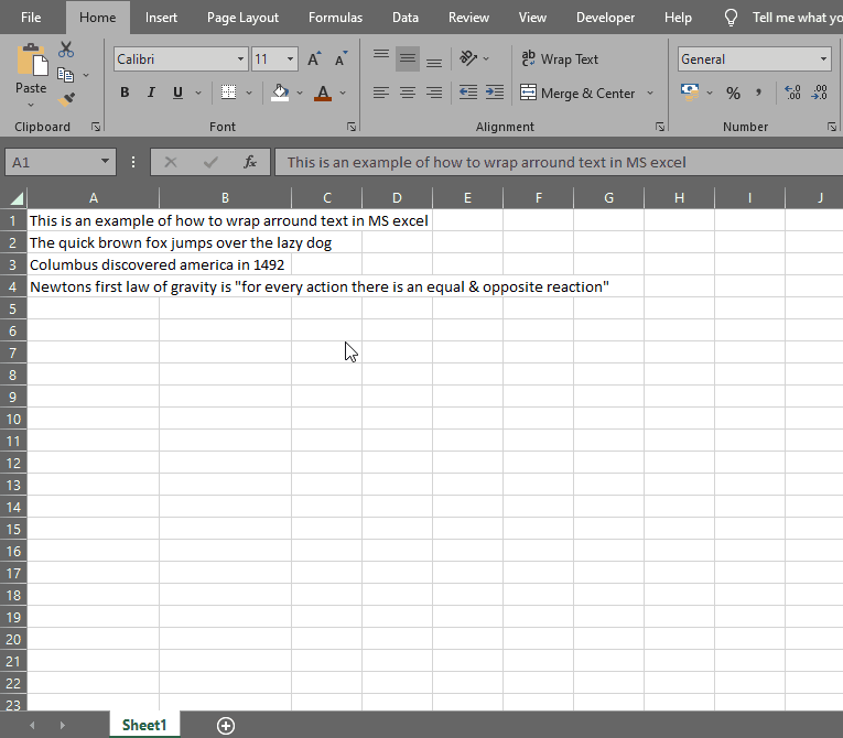
Step 1 – Select data range

• With the help of handle, select the data range.

Step 2 – Go To Home Tab

• Click on Home tab

Step 3 – Click Wrap Text Button

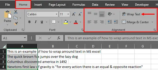
• In the Alignment group, click the Wrap Text button.

Step 4 – Get the wrapped text

• Your text will be wrapped automatically without disturbing column width.

Method 2 – Cell Formatting

Step 1 – Select data range

• With the help of handle, select the data range.

Step 2 – Go To Cell Formatting

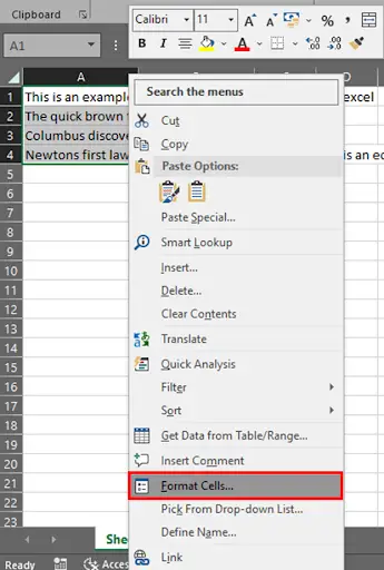
• Right mouse click on the selection

Step 3 – Format Cell Dialog Box

• Format Cells dialog will open. Switch to the Alignment tab, select the Wrap Text checkbox, and click OK.

Step 4 – Get the wrapped text

• Your text will be wrapped automatically without disturbing column width.

Method 3 – Shortcut Key

Step 1 – Select data range

• With the help of handle, select the data range.

Step 2 – Use of Shortcut Key

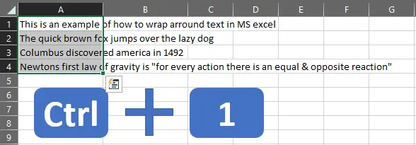
• After selecting the data, press Ctrl + 1 on your keyboard.

Step 3 – Format Cell Dialog Box

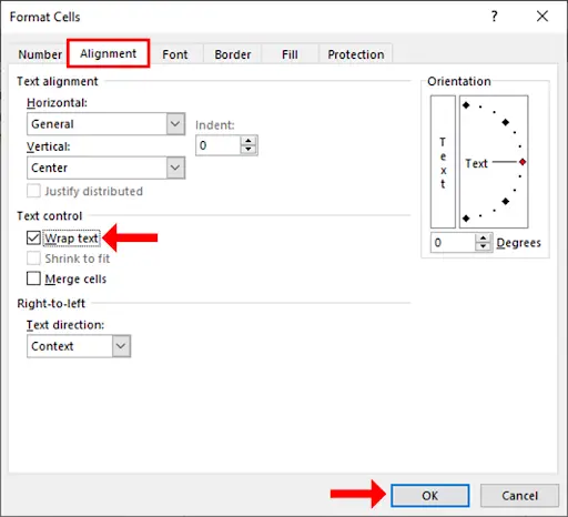
• Format Cells dialog will open. Switch to the Alignment tab, select the Wrap Text checkbox, and click OK.

Step 4 – Get the wrapped text

• Your text will be wrapped automatically without disturbing column width.

Whichever method you use, the data in the selected cells wraps to fit the column width. If you change the column width, text wrapping will adjust automatically.