
How to VLOOKUP and return multiple corresponding values vertically in Excel
 By
SpreadCheaters
By
SpreadCheaters
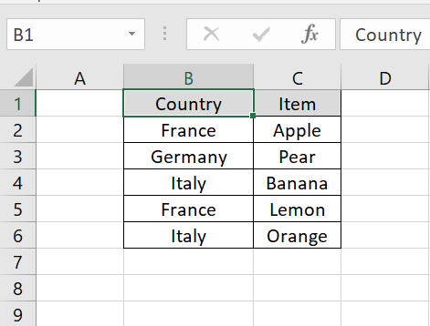
Here we have a dataset above, in this dataset, there are Countries and their Items related to fruits. In this tutorial, we will learn how to VLOOKUP values related to France and its Items but first let’s take a look at the Dataset. As discussed earlier, VLOOKUP only returns the first match it finds. To return multiple corresponding values vertically, you can use a combination of the INDEX, MATCH, and IF functions.
Here are the steps to perform a vertical VLOOKUP with multiple corresponding values:

Excel is a powerful tool for organizing and analyzing data, but sometimes you need to look up multiple corresponding values in a table. VLOOKUP is a commonly used function that helps to search and retrieve data from a table based on a lookup value. However, VLOOKUP only returns the first matching value it finds in a table, which can be limiting if you need to retrieve multiple values.
Step 1 – Select the value.
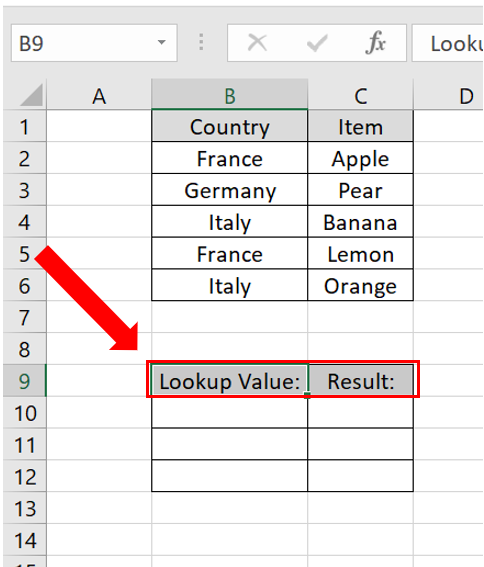
– Select the value you want to VLOOKUP in our case France.
– In a cell give the heading ‘Lookup Value’ and a cell with the heading ‘Result’ next to it.
Step 2 – Create the appropriate formula using INDEX, MATCH & IF
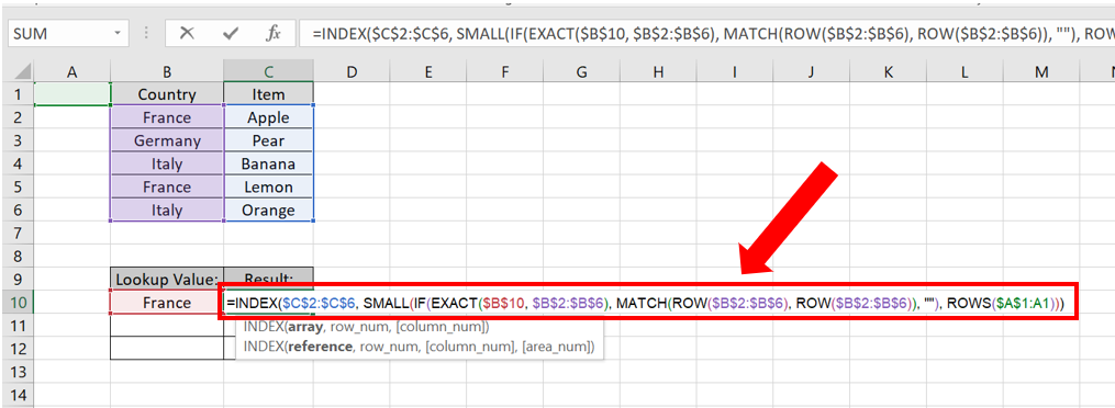
– In the Lookup Value column write the name of the value you want to look up in this case France.
– In the Result column enter the formula.
– In our case the formula will be
=INDEX($C$2:$C$6,SMALL(IF(EXACT($B$10,$B$2:$B$6), MATCH(ROW($B$2:$B$6), ROW($B$2:$B$6)), “”), ROWS($A$1:A1)))
Formula explanation is given in the last.
Step 3 – Implement the formula to search the values
– In order to enter the formula press Ctrl + Shift + Enter.
– Use the Fill Handle option to fill the other cells.
– The values will be displayed.
Formula Explanation:
=INDEX($C$2:$C$6, SMALL(IF(EXACT($B$10, $B$2:$B$6), MATCH(ROW($B$2:$B$6), ROW($B$2:$B$6)), “”), ROWS($A$1:A1)))
=INDEX($C$2:$C$6), This specifies the array from which to return a value. In this case, it’s the range C2:C6.
SMALL(IF(EXACT($B$10, $B$2:$B$6), MATCH(ROW($B$2:$B$6), ROW($B$2:$B$6)), “”), ROWS($A$1:A1))) This is the part that generates an array of values that the INDEX function will use to return a result.
IF(EXACT($B$10, $B$2:$B$6), MATCH(ROW($B$2:$B$6), ROW($B$2:$B$6)), “”) This generates an array of row numbers for which the value in column B matches the value in cell B10. If there’s a match, it returns the row number; otherwise, it returns an empty string.SMALL(array, ROWS($A$1:A1)) This returns the kth smallest value from the array. The k value is determined by the number of rows in the reference ($A$1:A1), which increases by 1 as the formula is copied down. As a result, the formula returns the first, second, third, etc. smallest values from the array.


