
How to use XMATCH function in Excel
 By
SpreadCheaters
By
SpreadCheaters
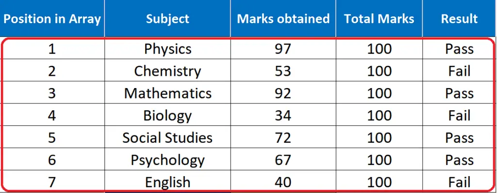
In this tutorial we’ll learn how to use XMATCH by implementing this function to search within a real data set.
As we discussed earlier XMATCH is a successor of MATCH function therefore, it has all the capabilities of MATCH function. However, it has some more flexibility and offers more ways to search the data. We’ll explore all of them.
Syntax of XMATCH
First of all we will take a look at the syntax of the XMATCH function in order to understand how to write the function and what parameters it will accept. So the syntax of this function is as follows;
=XMATCH (lookup_value, lookup_array, [match_mode], [search_mode])
lookup_value:
It is the value that will be searched.
lookup_array:
It is the range of data in which the lookup value will be searched
[match_mode]:
This is an optional parameter which will tell Excel how to search the array. This is where the XMATCH function differs from the MATCH function. XMATCH has four options while the MATCH function has only three options here.
0 = Exact match (which is the default option)
-1 = Exact match or next smallest
1 = Exact match or next largest
2 = Wildcard match
[search_mode]:
This mode is also a difference between XMATCH & MATCH functions, because this is available only in XMATCH. It has four options as well.
1 = search from first (default)
-1 = search from last
2 = binary search ascending
-2 = binary search descending
XMATCH function can look up a value in an array in horizontal or vertical and return the index for the position of the lookup value. It can lookup for exact or partial matches, supports wildcards, can search both in forward and reverse directions and also offers the binary search options which are added for speed optimization of searches.
Let’s explore the match modes and search modes of this function step by step.
Excel provides us with a lot of formulas and built-in functions which can be used to search big data sets within seconds. One such function is XMATCH. This function is a successor of the MATCH function and works in almost the same way with some differences.
Step 1 – Lookup for Exact Match
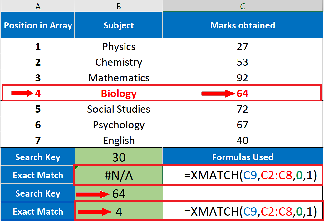
– To find an exact match the following formula will be used;
=XMATCH(C9,C2:C8,0,1) for exact match only
– We used “0” in the search mode option which tells the formula to look for exact matches. We searched for two values, 30 and 64. The first one was not available in the array so we got #N/A error. However, 64 was available at 4th position in the array as shown in the picture above so we got 4 as the result of the second search.
Step 2 – Lookup for Next Smallest and Next Largest Matches
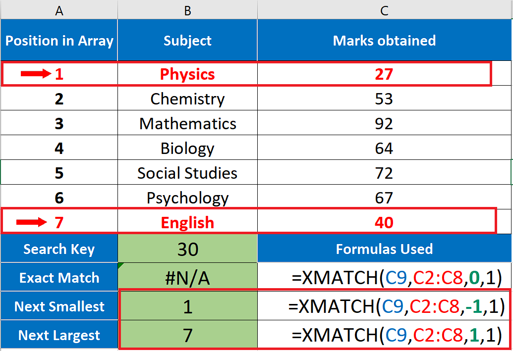
– To find next smallest and next largest matches the following formulas will be used;
=XMATCH(C9,C2:C8,-1,1) for next smallest
=XMATCH(C9,C2:C8,1,1) for next largest
– We used “-1” in the search mode option in the first formula which tells the formula to look for the exact or next smallest match. The search key in this case was 30 which was not available in the array so the first formula looked for the next smallest number. Therefore, we got 1 as the result of the search, which is actually the position of number 27 in the array.
– We used “1” in the search mode option in the first formula which tells the formula to look for the exact or next largest match. The search key in this case was 30 which was not available in the array so the first formula looked for the next largest number. Therefore, we got 7 as the result of the search, which represents number 40 in the array.
Step 3 – Lookup for Next Smallest and Next Largest Matches
– To find next smallest and next largest matches the following formulas will be used;
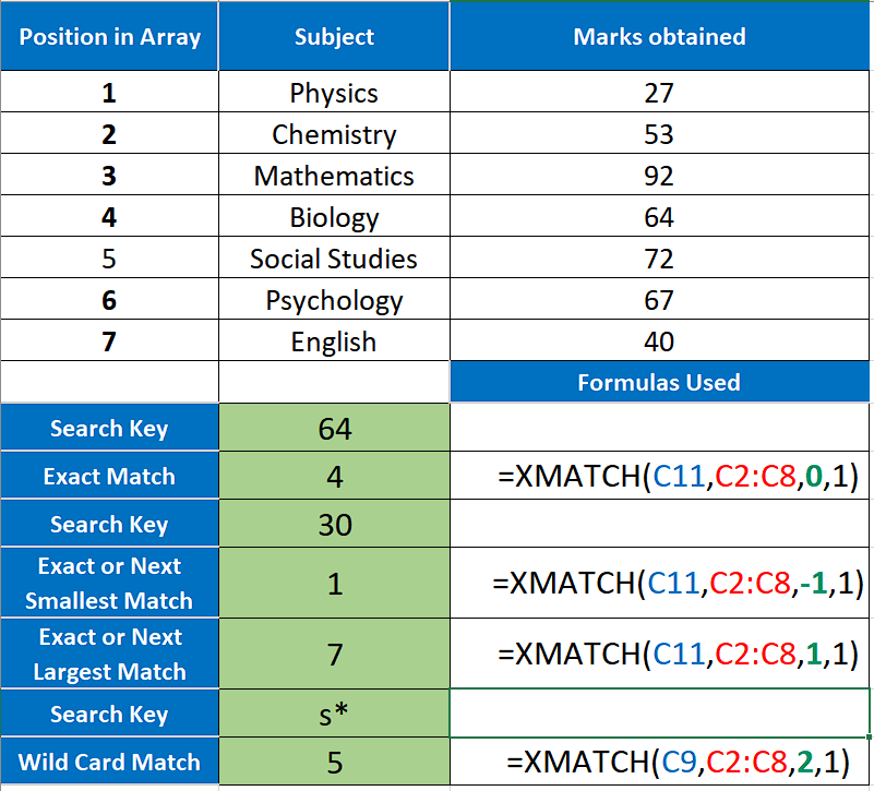
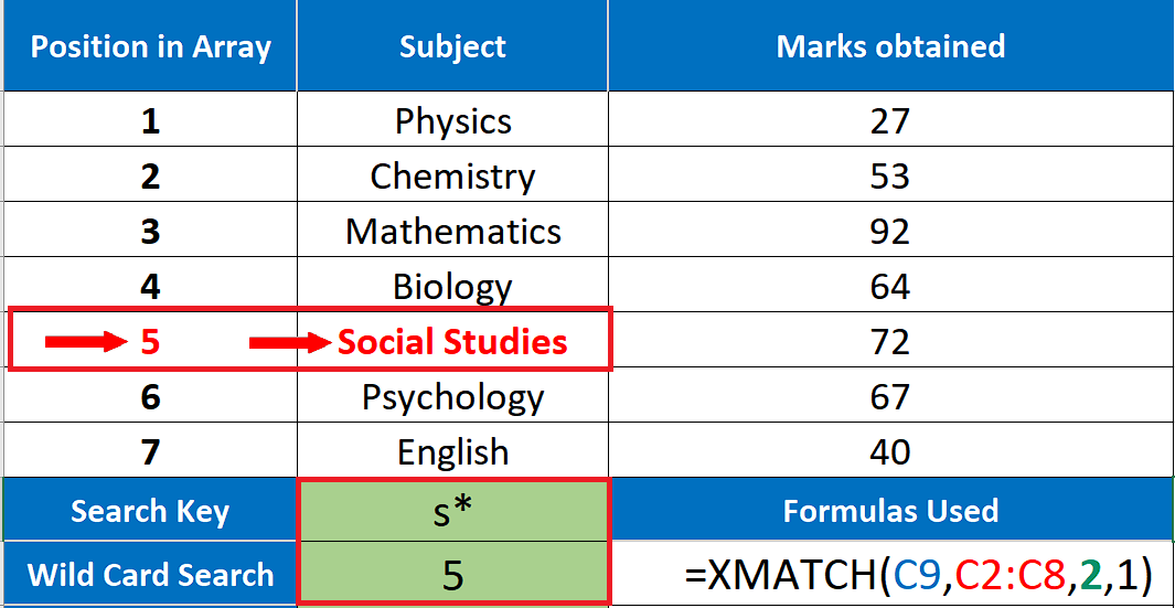
=XMATCH(C9,C2:C8,2,1) for wild card matches
– We used “2” (search with wildcard) in the search mode option in the formula which tells the formula to look for the word starting with letter s (case in-sensitive). So the first formula found the word Social Studies and returned 5 as the result of the search, which represents the position of Social Studies in the array.
So this is how we can use XMATCH to find the indices of the numbers or any other search key in the range of data.


