How To Use XLOOKUP In Excel With Two Sheets
The XLOOKUP function has several advantages over its predecessors, including the ability to search for values in any column, not just the first column of a table. It can also perform approximate matches and wildcard matches, and return an array of results.
Let’s understand the function first, then use it in our example.
For this example, we’ll be working with two sheets: Sheet1 and Sheet2. Sheet1 contains a list of employee names and their corresponding email addresses, while Sheet2 contains a list of employee names and their corresponding department.
We will use Xlookup function to find out Employee email address from sheet 1.

The XLOOKUP function in Excel is a powerful search and lookup function that allows you to search for a specific value in a table or range of cells, and return a corresponding value in another column. It is an improved version of the VLOOKUP and HLOOKUP functions.
Step 1 – Start The XLOOKUP Function

– Start typing the XLOOKUP function by typing an equal sign (=), followed by “XLOOKUP”.
Step 2 – Enter The Lookup Value

– The first argument for the XLOOKUP function is the lookup value. In this case, we want to use the employee name in cell A2 of Sheet2.
– So after the opening parenthesis, type “A2”, and then a comma.
Step 3 – Specify the Lookup Array
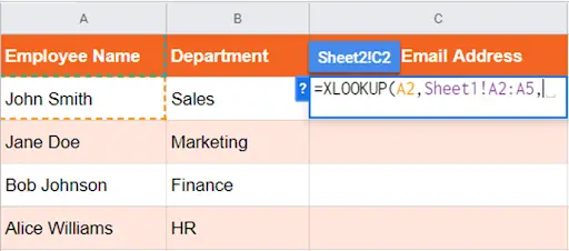
– The second argument for the XLOOKUP function is the lookup array. This is the range of cells that contains the values you want to search for the lookup value.
– In this case, the lookup array is the range of employee names in Sheet1 (A2:A5).
– So after the comma, type “Sheet1!A2:A5”, and then a comma.
Step 4 – Specify the Return Array
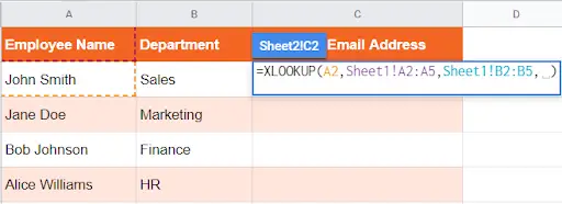
– The third argument for the XLOOKUP function is the return array. This is the range of cells that contains the values you want to return when a match is found.
– In this case, the return array is the range of email addresses in Sheet1 (B2:B5).
– So after the comma, type “Sheet1!B2:B5”, and then a comma.
Step 5 – Specify the Match Mode
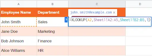
– The fourth argument for the XLOOKUP function is the match mode. This specifies how the lookup value should be matched against the values in the lookup array.
– In this case, we want an exact match, so we’ll use “1”.
– So after the comma, type “1”, and then a closing parenthesis.
Step 6 – Press Enter
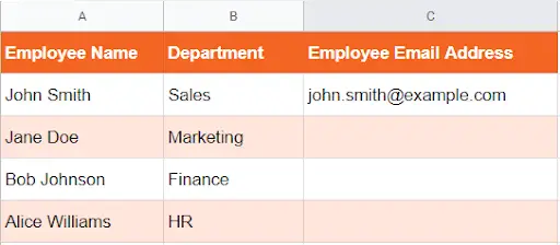
– Press Enter, and the email address for John Smith should appear in cell C2.
Step 7 – Drag The Formula Downwards
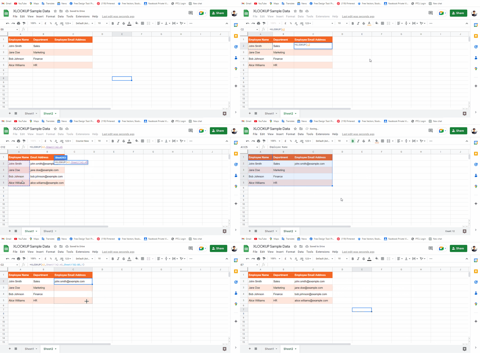
– Drag the formula to the remaining cells of your table.


