
How to use Vlookup in Excel to compare two columns
 By
SpreadCheaters
By
SpreadCheaters
You can watch a video tutorial here.
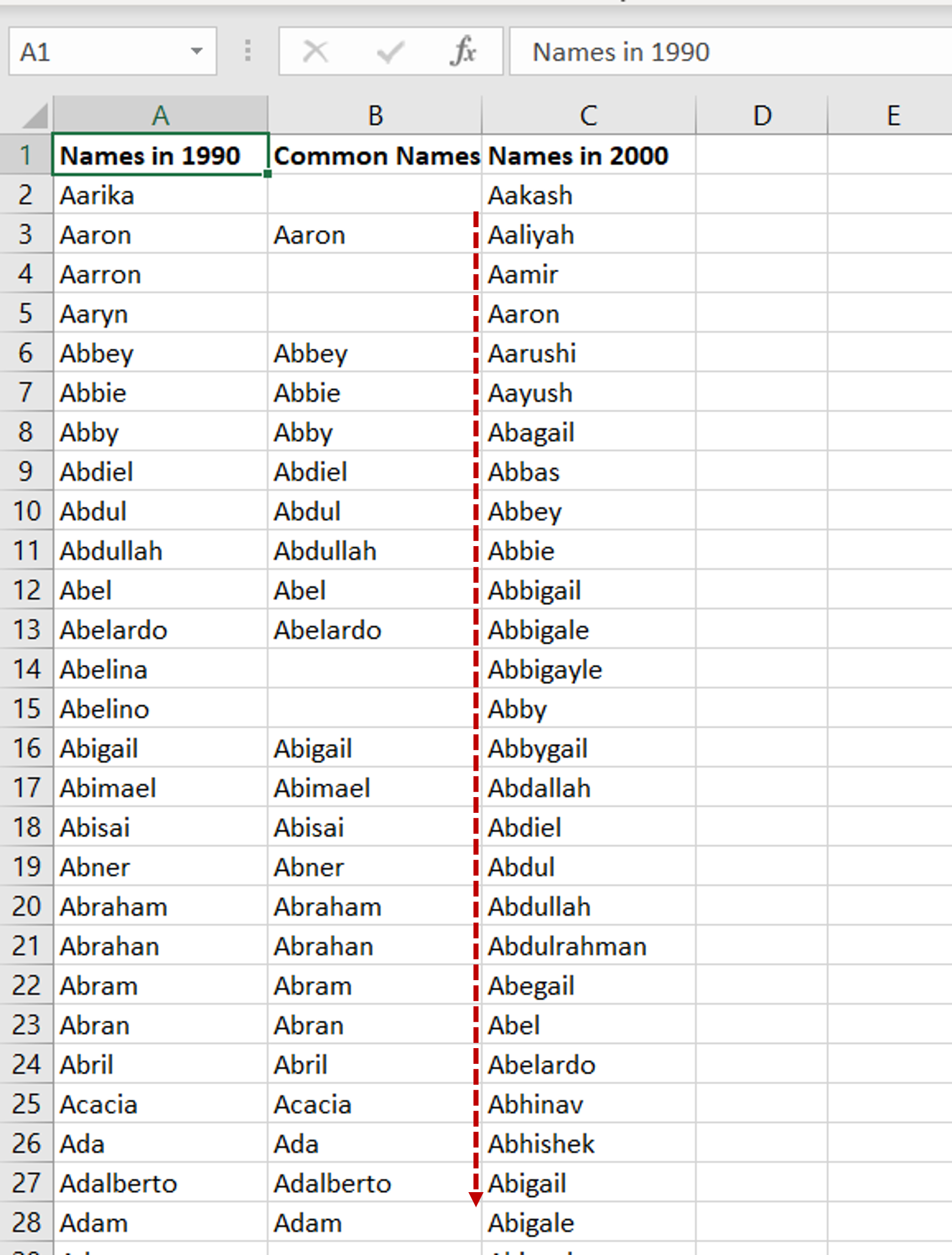
Vlookup is one of the most useful functions in Excel when it comes to comparing data from multiple columns. As long as the columns share a column field or ‘key’, data from both columns can be easily compared. In this example, we want to see which names from the year 1990 were used again in the year 2000. Here the key is the name.
Step 1 – Open the Formula wizard
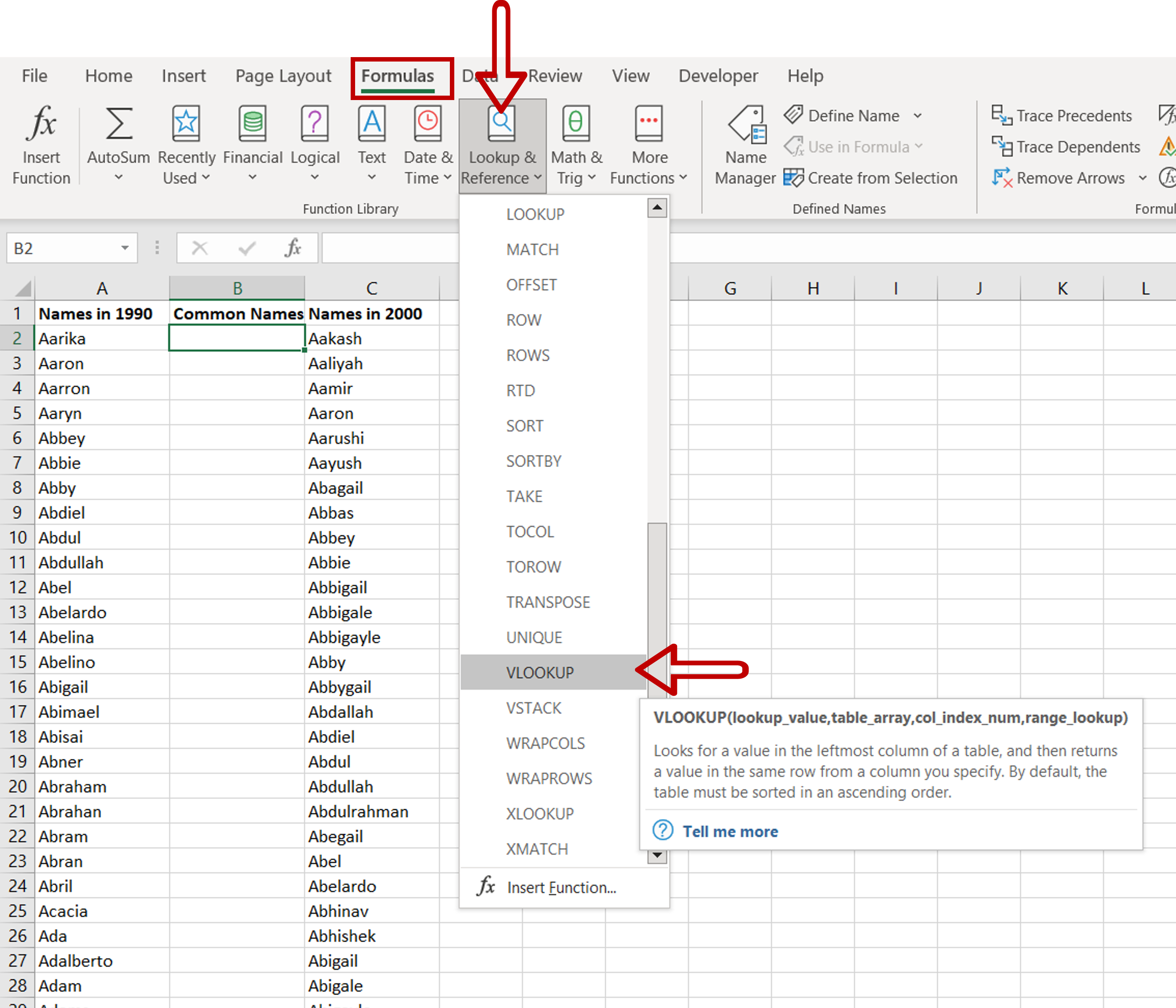
– Select the destination cell
– Go to the Formulas > Lookup & Reference > Vlookup
– The data from 1990 will be Table 1 and the data from 2000 will be Table 2
Note: A few things to keep in mind when using Vlookup:
>The key must always be in the left-most column of Table 2
>Table 2, or the table that is being referred to must always be sorted on the key, in ascending order
>It is better Table 2 has unique values or else this function may not return the desired result
Step 2 – Enter the arguments for the VLOOKUP() function
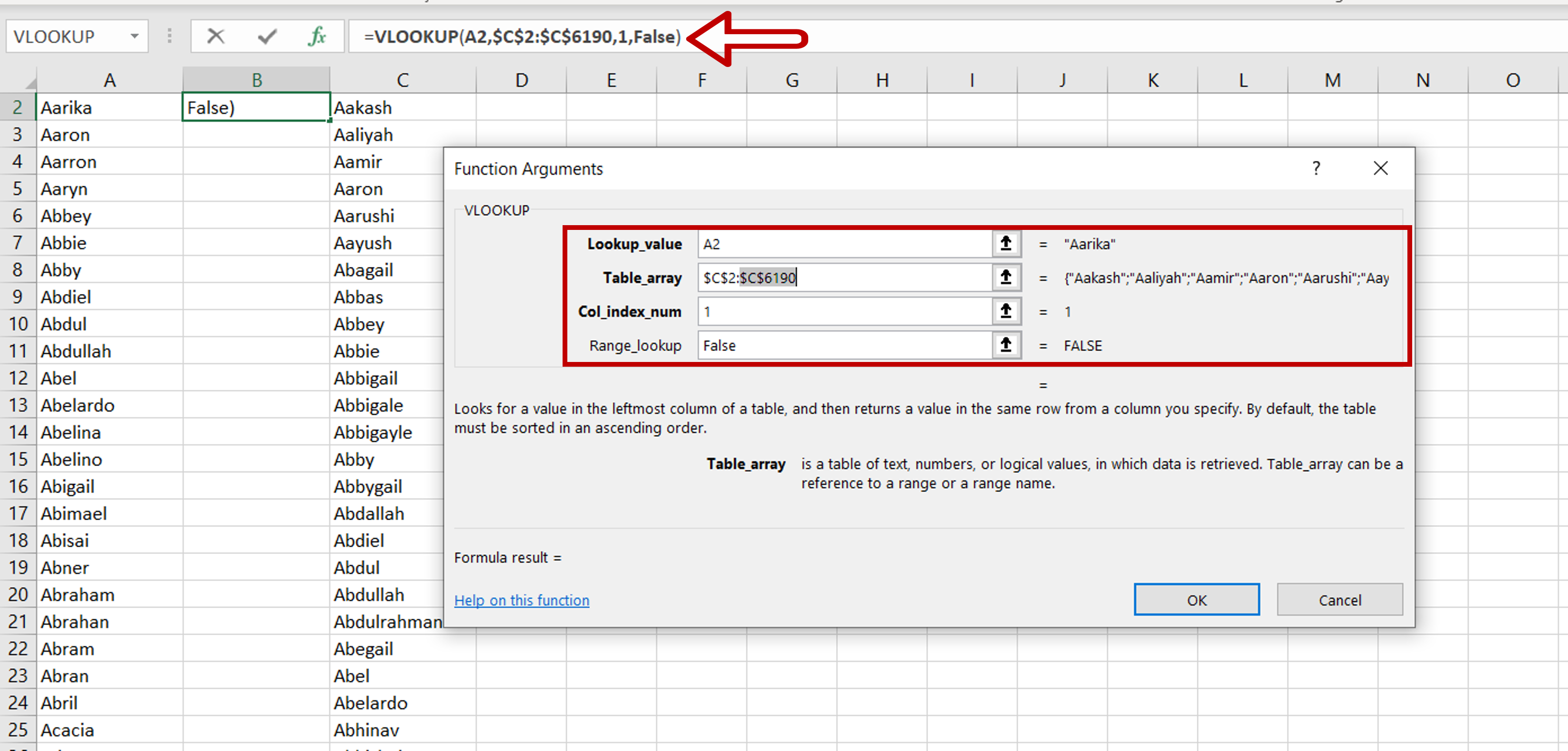
– Lookup value: the cell reference of the first value in the key column from Table 1 (Name)
– Table-array: the range of Table 2 which is made constant with the addition of dollar signs ($)
– Col_index_num: the number of the column in Table 2 that has to be retrieved (1 i.e. the Name)
– Range_lookup: TRUE will return an approximate match, FALSE will return an exact match
– Click OK
Step 3 – Enhance the formula to handle errors i.e. missing values
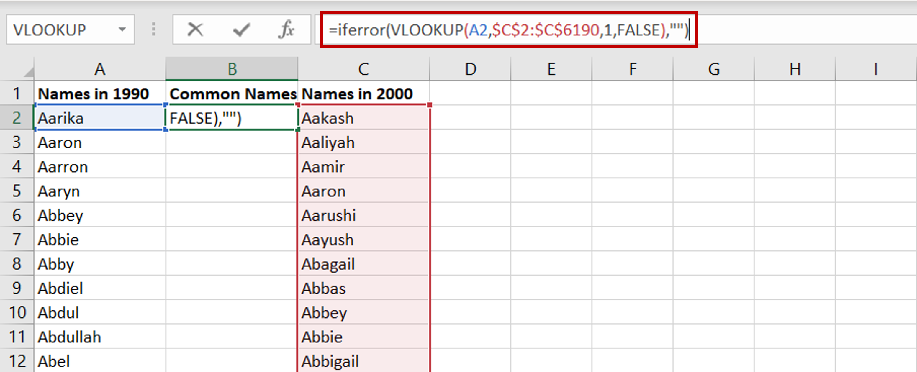
– If the lookup function cannot find a match in Table 2 i.e. the name is not present in Table 2, an error message is returned – #N/A
– Change the formula to display an empty cell if a match cannot be found:
= iferror(<vlookup formula>,0)
Step 4 – Copy the formula
– Using the fill handle from the first cell, drag the formula to the remaining cells
OR
a) Select the cell with the formula and press Ctrl+C or choose Copy from the context menu (right-click)
b) Select the rest of the cells in the column and press Ctrl+V or choose Paste from the context menu (right-click)
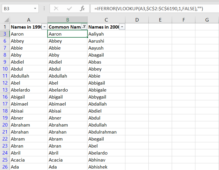
Step 5 – Filter the data
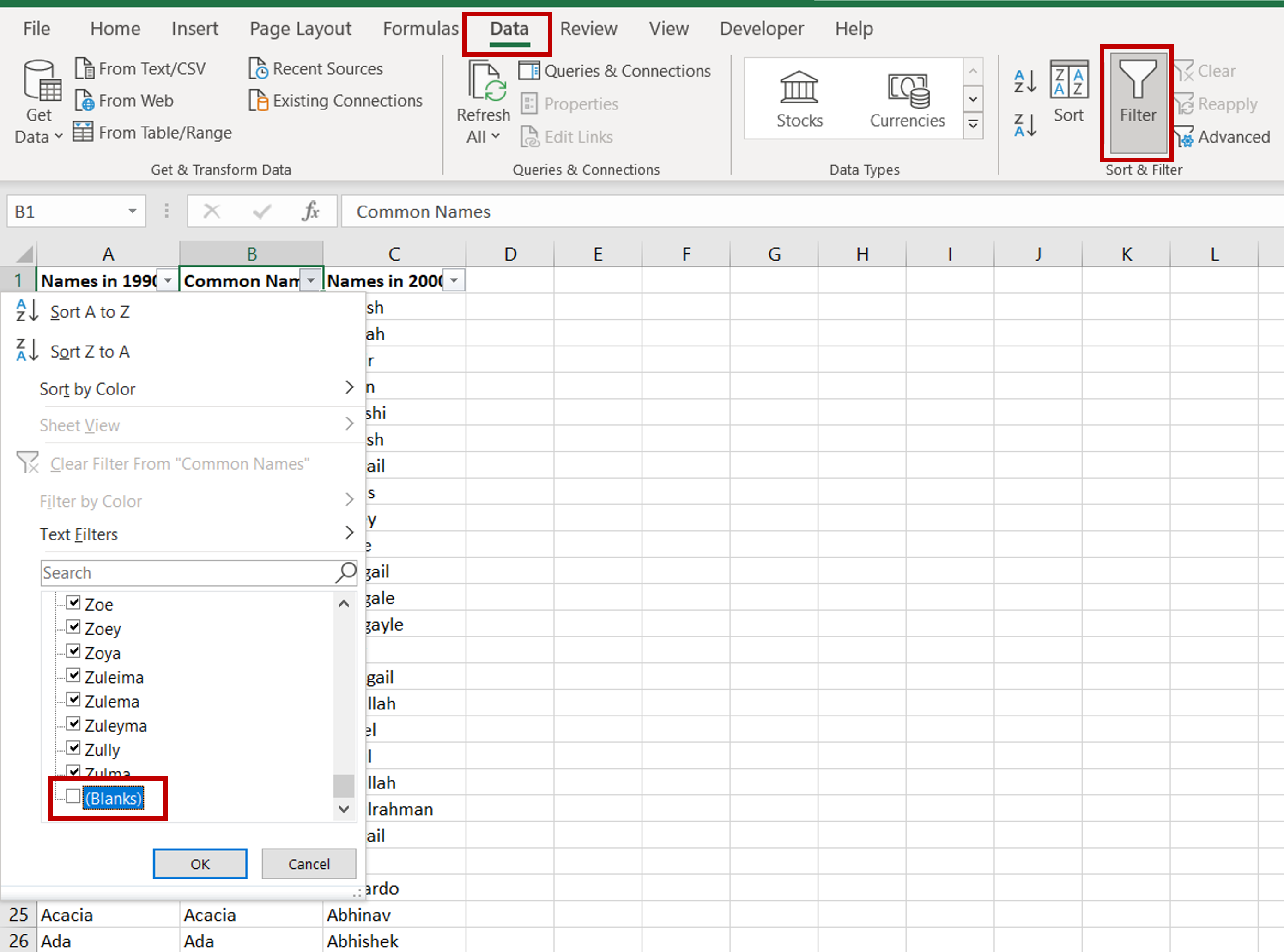
– Go to Data > Sort & Filter
– Press the Filter button
– From the in-column filter, scroll down and remove (Blanks)
– Click OK
Step 6 – Check the data
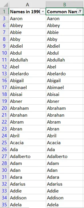
– Check the data


