
How to use the cell function in Excel
 By
SpreadCheaters
By
SpreadCheaters
Excel has a function called CELL, which gives us various information aboutthe cell. The type of information which will be received is known as info_type. The CELL function can get things like address and filename, as well as detailed info about the formatting used in the cell. The complete list of the type of information that this function can return is given in the table below.
| Info_type | Description |
|---|---|
| address | returns the address of the first cell in reference (as text). |
| col | returns the column number of the first cell in reference. |
| color | returns the value 1 if the first cell in reference is formatted using color for negative values; or zero if not. |
| contents | returns the value of the upper-left cell in reference. Formulas are not returned. Instead, the result of the formula is returned. |
| filename | returns the file name and full path as text. If the worksheet that contains reference has not yet been saved, an empty string is returned. |
| format | returns a code that corresponds to the number format of the cell. See below for a list of number format codes. If the first cell in reference is formatted with color for values < 0, then “-” is appended to the code. If the cell is formatted with parentheses, returns “() – at the end of the code value. |
| parentheses | returns 1 if the first cell in reference is formatted with parentheses and 0 if not. |
| prefix | returns a text value that corresponds to the label prefix – of the cell: a single quotation mark (‘) if the cell text is left-aligned, a double quotation mark (“) if the cell text is right-aligned, a caret (^) if the cell text is centered text, a backslash () if the cell text is fill-aligned, and an empty string if the label prefix is anything else. |
| protect | returns 1 if the first cell in reference is locked or 0 if not. |
| row | returns the row number of the first cell in reference. |
| type | returns a text value that corresponds to the type of data in the first cell in reference: “b” for blank when the cell is empty, “l” for label if the cell contains a text constant, and “v” for value if the cell contains anything else. |
| width | returns the column width of the cell, rounded to the nearest integer. A unit of column width is equal to the width of one character in the default font size. Note: this value comes back as an array with two values {width,default} where width is the column width and default is a boolean value that indicates if the width is the default column width. |
We’ll cover some of the most useful features of these info_type and explain how they can be used. Let’s explore the usage of some of the features of this function in the steps below.
Excel has very powerful features for calculations and data manipulation. While working with different data types in Excel, it is mandatory to get some specific information about the data cells. Cells are the data storing blocks in Excel. In very simple words, we can say that each box in Excel is a cell that can store data.
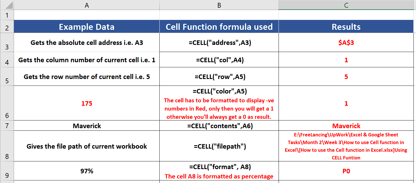
Step 1 – Get the absolute address of the reference Cell
– To get the absolute reference of any cell we can use the following formula,
=CELL(“address”, A3)
This will give us the address of A1 in the cell where we applied the formula as shown above.
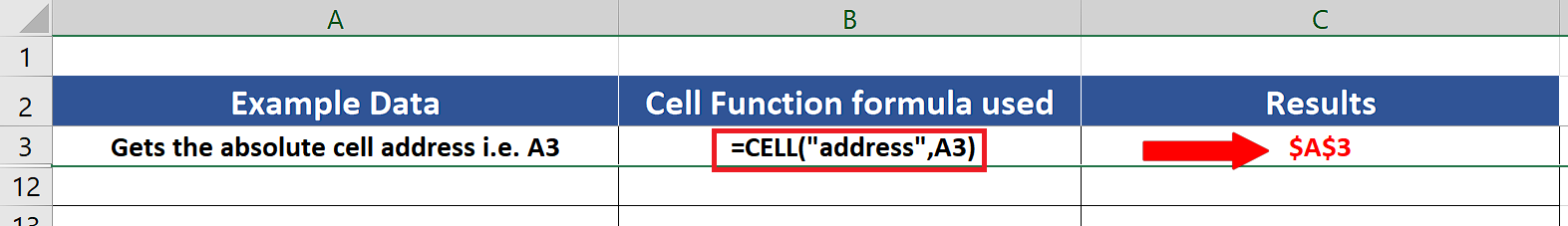
Step 2 – Get the column or row number of the reference Cell
– To get the row or column number of any cell we can use the following formula,
=CELL(“col”, A4)
=CELL(“row”, A5)
This will give us the row number of A4 and column number of A5 in the cell where we applied the formula as shown above.
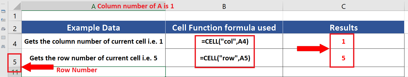
Step 3 – Know if the reference Cell is formatted to show negative numbers in red color
– By using the CELL function, we can know if the cell is formatted to display negative numbers in red or not. This is a special technique used by some data analysts, in which the negative numbers are shown as positive but their font color is changed to red to indicate that actually the number in consideration is a negative number. So we’ll use the following formula for this one
=CELL(“color”,A5)
Step 4 – Get the contents of the reference Cell
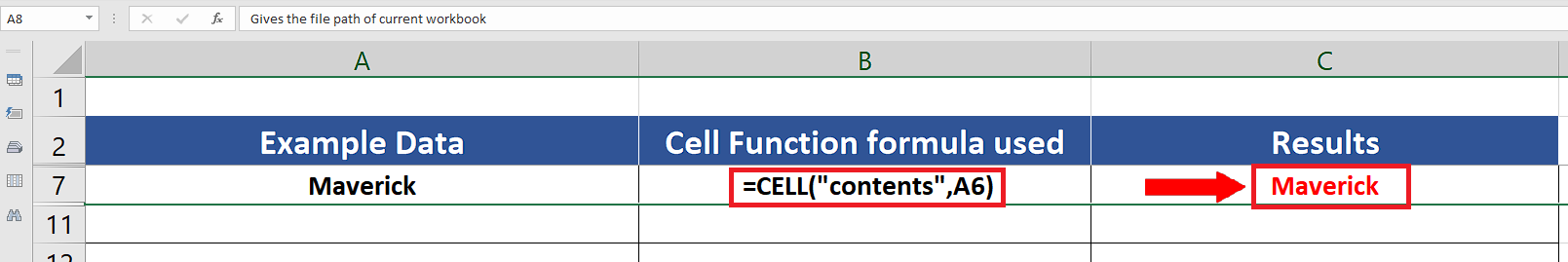
– We can get the contents of any cell by using this feature. However, to get the contents of the cell A6 we can use the following formula,
=CELL(“contents”, A6)
This will give us the contents of A6 in the cell where we applied the formula as shown above.
Step 5 – Get the complete file path of the current workbook
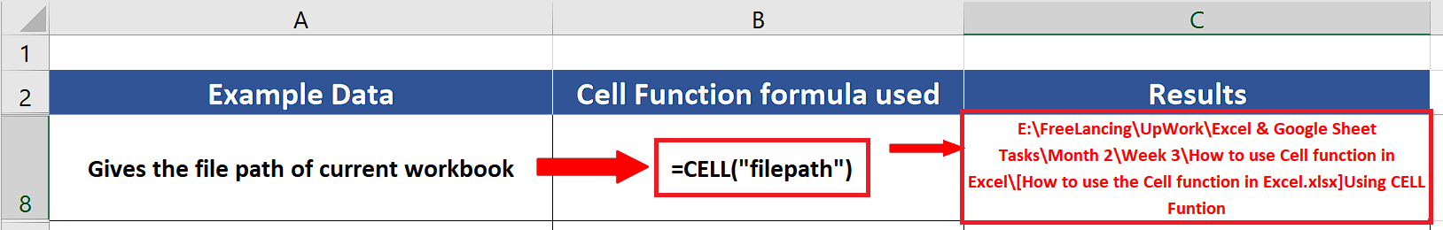
– We can get the complete path of the current worksheet in any cell. For this purpose, we can use the following formula,
=CELL(“filepath”)
This will give us the complete file path including the name of the currently Active worksheet in the cell where we applied the formula as shown above.
Step 6 – Get the format details of data in the reference cell
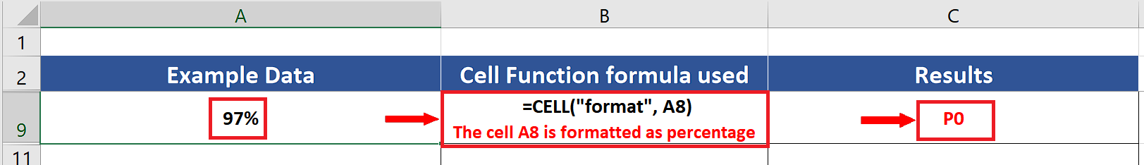
– We can get the details of the format of the data in any cell through the CELL function. For this purpose, we can use the following formula,
=CELL(“format”, A9)
This will give us the details of the data format of cell A9 in the cell where we applied the formula as shown above.
The format will be shown as a code number and the details of the code numbers are given below;
Format codes
The table below shows the text codes returned by CELL when “format” is used for info_type.
| Format code | Format code meaning | Format code | Format code meaning |
|---|---|---|---|
| G | General | S2 | 0.00E+00 |
| F0 | 0 | G | # ?/? or # ??/?? |
| ,0 | #,##0 | D1 | d-mmm-yy or dd-mmm-yy |
| F2 | 0 | D2 | d-mmm or dd-mmm |
| ,2 | #,##0.00 | D3 | mmm-yy |
| C0 | $#,##0_);($#,##0) | D4 | m/d/yy or m/d/yy h:mm or mm/dd/yy |
| C0- | $#,##0_);[Red]($#,##0) | D5 | mm/dd |
| C2 | $#,##0.00_);($#,##0.00) | D6 | h:mm:ss AM/PM |
| C2- | $#,##0.00_);[Red]($#,##0.00) | D7 | h:mm AM/PM |
| P0 | 0% | D8 | h:mm:ss |
| P2 | 0.00% |


