How to use SUM with INDEX-MATCH Function in Excel

That’s exactly what we will be teaching to you today in this Step-by-Step Tutorial. We have a data set of a Mobile store showing sales of different mobile brands and their specific models. We will be using SUM, INDEX, and MATCH functions to calculate the total sales of some specific models in the past five months.

SUM FUNCTION

The SUM function is used to add a set of numbers together. It is one of the most fundamental and widely used functions in Excel. The SUM function can add up individual numbers, a range of cells, or a combination of both. Its syntax is very basic:

Syntax =SUM(number1, [number2], …)

INDEX FUNCTION

In Excel, the INDEX function is used to return the value of a cell in a specified row and column within a range of cells. The INDEX function can be used to create dynamic references, such as retrieving data from a table based on the value in another cell. It is also commonly used in Excel lookups in combination with the MATCH function. Following is the syntax of the INDEX function:

=INDEX(array, row_num, [column_num])

OR

=INDEX(reference, row_num, [column_num], [area_num])

MATCH FUNCTION

The MATCH function in Excel is used to find out the relative position of a value within a range of cells and returns that position as a row or column number. The function searches the range for the specified value and returns the relative position of the value’s first occurrence. The MATCH function returns an error if the value is not found in the range.

Syntax =MATCH(lookup_value, lookup_array, [match_type])

Nesting SUM function with INDEX-MATCH function in Excel

The INDEX and MATCH functions can be combined. It works well to extract specific data from a big array. The row and column positions of the input values are what the MATCH function looks for and the INDEX function simply returns the result of the intersection of the row and column positions. The SUM function will then return the sum of the found values. We can also integrate this INDEX-MATCH function into SUM or SUMPRODUCT function as well.

Following is one of the possible criteria;

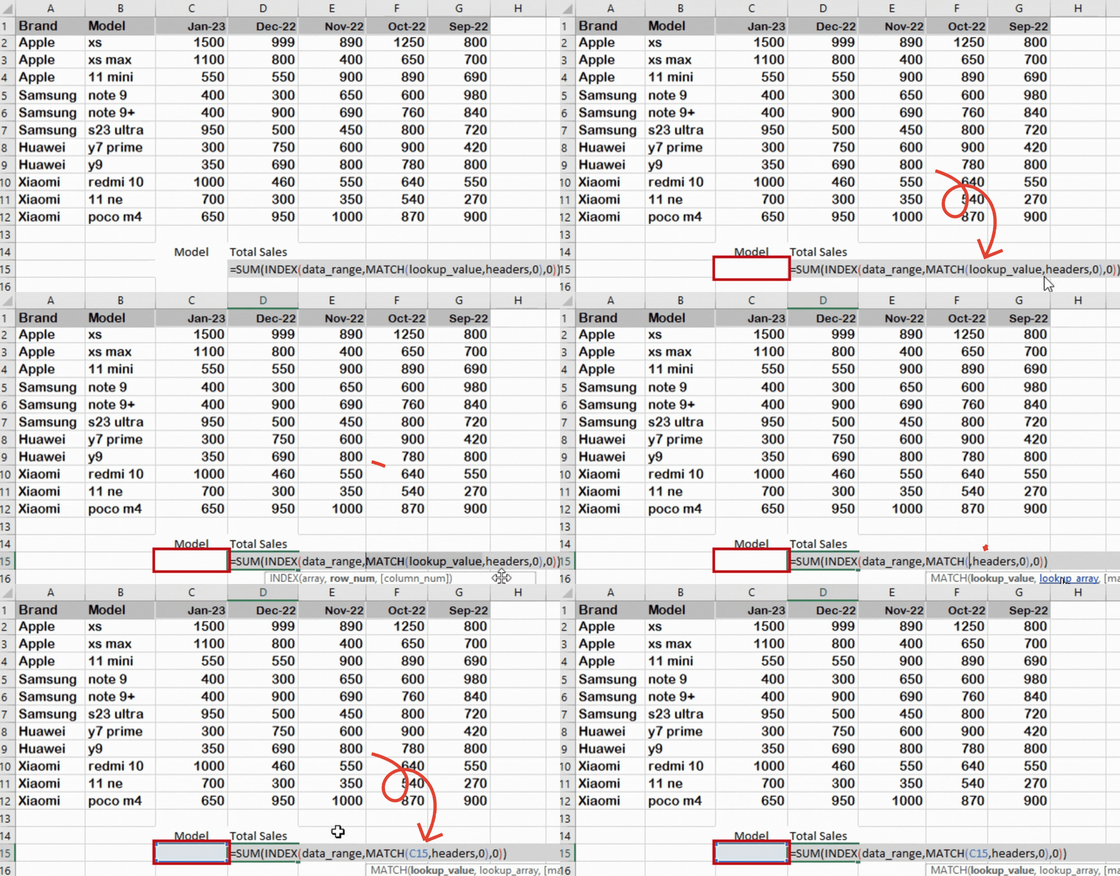
=SUM(INDEX(data_range,MATCH(lookup_value,headers,0),0))

Where;

data_range:

This is the selected range of data on which you want to perform calculations.

lookup_value:

This function refers to a cell to match values in another row or column against the cell and thereby retrieving the corresponding results from the respective rows and columns.

Microsoft Excel is a spreadsheet program that has a lot of functions to perform various data manipulations. Functions are used in Excel to perform different calculations. Excel functions can be combined to perform multiple tasks and calculations in a single formula. This helps to streamline processes and saves time by allowing users to perform multiple operations in a single step.

Step 1 – Add Look_Up Value

– Write the following formula in an appropriate cell 
=SUM(INDEX(data_range,MATCH(lookup_value,headers,0),0))

– Enter the lookup_value on which you want to search for in the data range.

– In our case, we’ll use a cell C15 and the formula will look up for any model number entered in cell C15

– So, our formula will become 
=SUM(INDEX(data_range,MATCH(C15,headers,0),0))

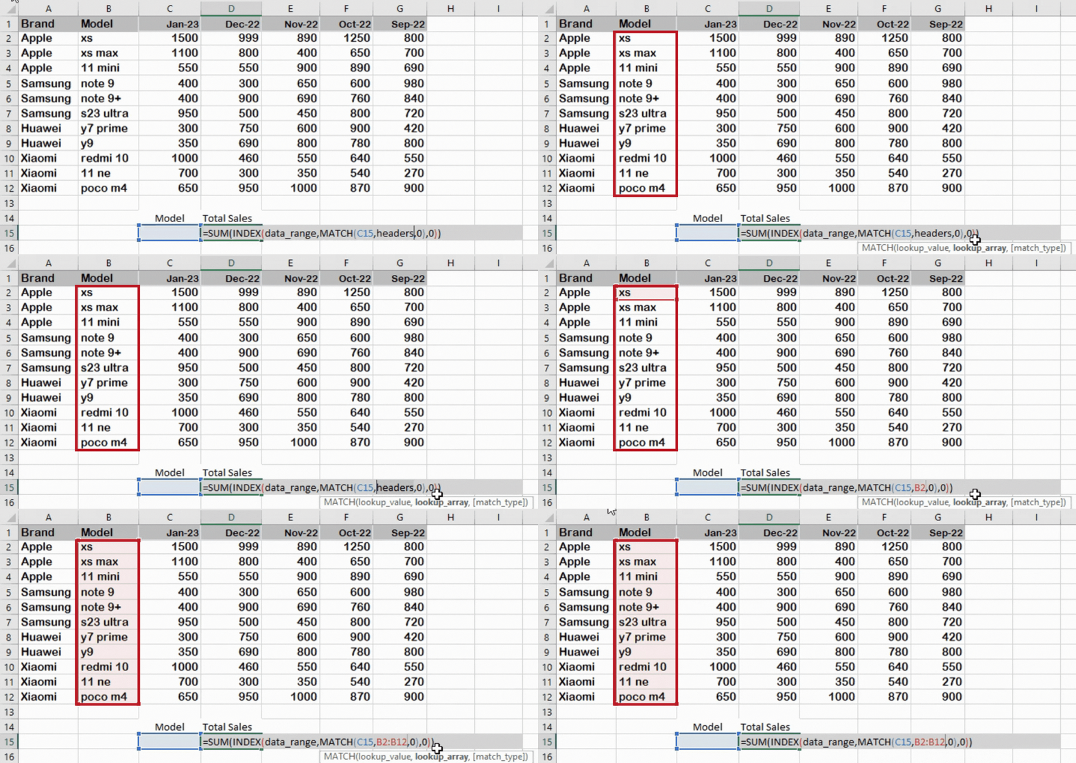
Step 2 – Add Headers Value

– Now we’ll choose the headers range. This will be the array in which the lookup value will be searched for, which in our case is B2:B12. The model names of all mobiles are in this column. So, write the following in the formula:

=SUM(INDEX(data,MATCH(C15,B2:B12,0),0))

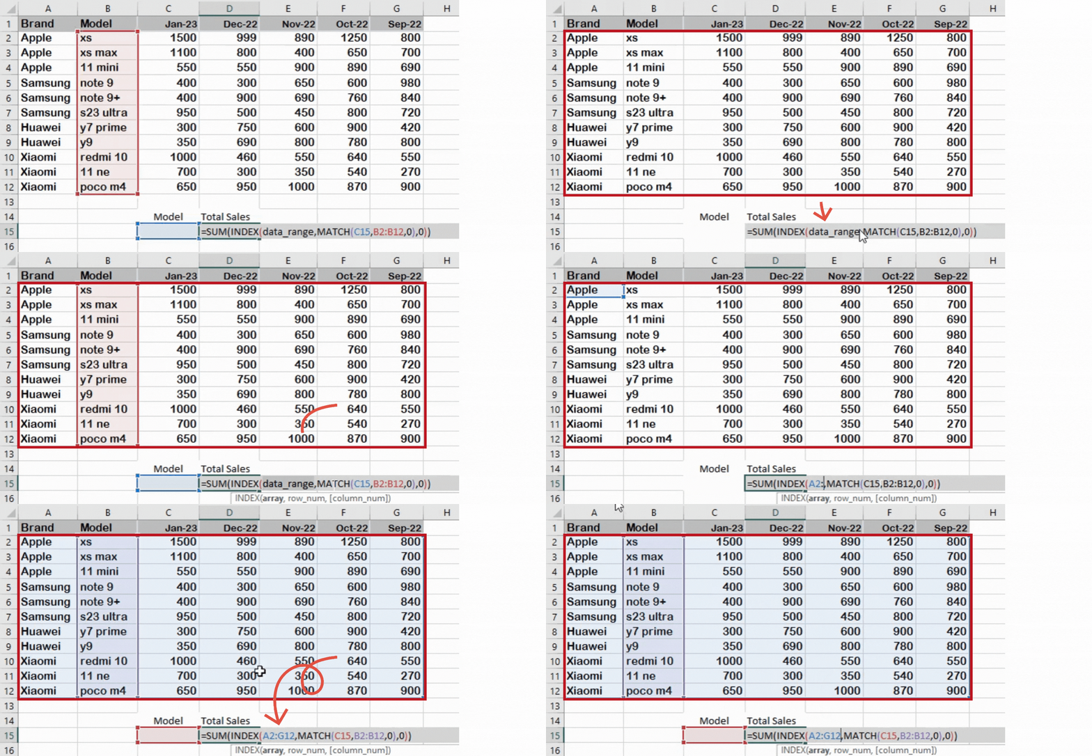
Step 3 – Select the Data Range

– Now, we’ll enter the data_range in the following formula, this will be the range of cells having the data on which the calculations will be performed. In our case, it’s A2:G12.

– Enter the following in the formula
=SUM(INDEX(A2:G12,MATCH(C15,B2:B12,0),0))

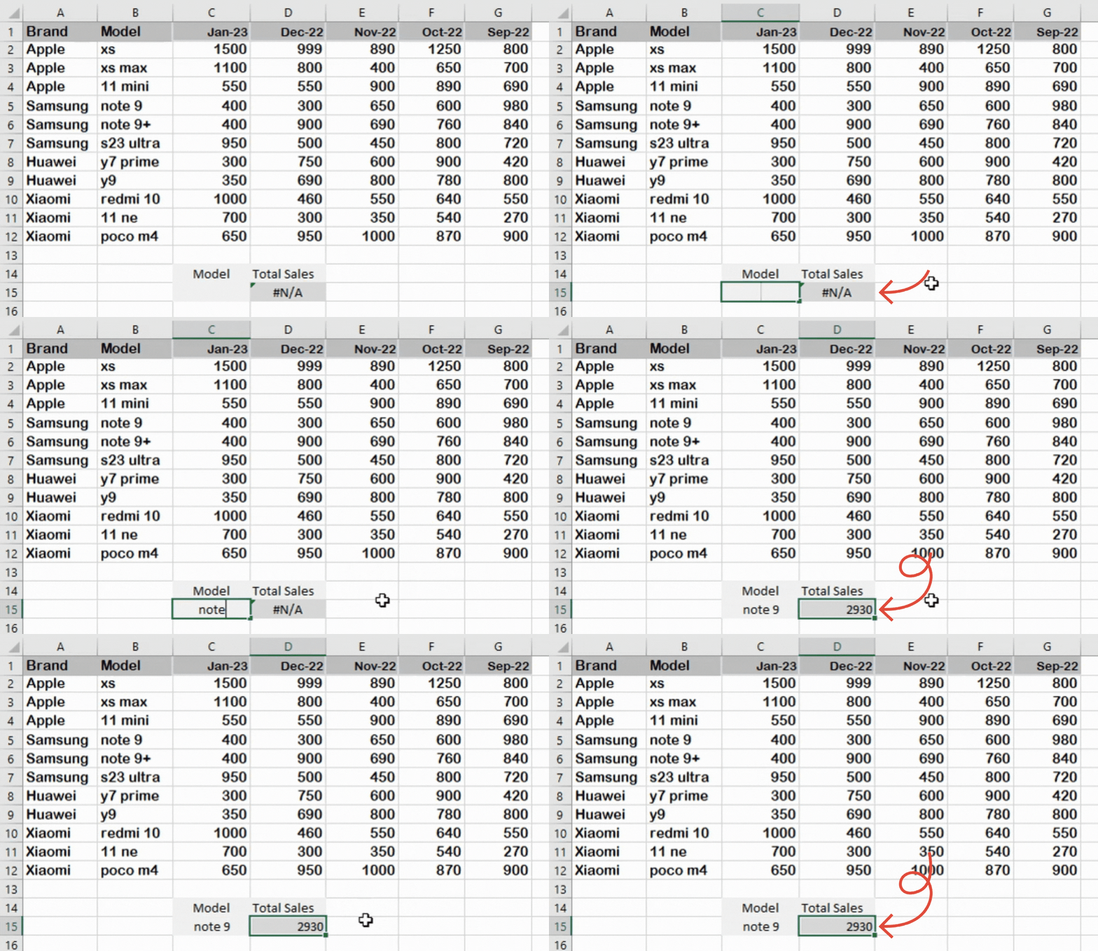
Step 4 – Enter the ‘Model number’ in the cell C15

– =SUM(INDEX(A2:G12,MATCH(C15,B2:B12,0),0))

After completing the whole formula, All we have to do is to enter the Model number whose sales you want to calculate in the lookup_value cell ‘C15’.

– Here, I am calculating total sales for the specific model ’note 9’.

– After entering the model number, press the ‘Enter’ button.

– Doing this will calculate total sales of note 9 in the past five months.

As you can see in the above animation, we got the Sum of the total sales of ‘note 9’ in the past five months. This formula =SUM(INDEX(A2:G12,MATCH(C15,B2:B12,0),0)) is generic,

Excel will automatically calculate the total sales of any entered model. I hope you understand how to use the SUM with INDEX and MATCH Functions in Excel.