How To Use Subtotal With Countif Condition In Excel

One thing is very important to know that the function SUBTOTAL is normally used to operate on a filtered dataset. We can then apply many possible operations on the filtered data using SUBTOTAL e.g., SUM, COUNT, AVERAGE etc. However, SUBTOTAL can’t be used in conjunction with COUNTIF, because COUNTIF returns only a single number and SUBTOTAL requires an array of data. Therefore, we need to achieve the task with some workaround for this.

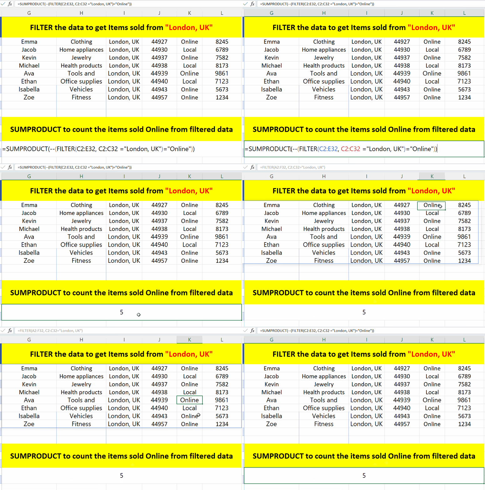
Let’s take a look at the following dataset above consisting of names, products names, shipping locations, shipping dates along with their channel of selling i.e., Online and Local. This dataset will be used as an example for learning today’s tutorial and we’ll try to find out the count of all those products which are sold from London, UK through the online channel.

As discussed earlier SUBTOTAL can’t be used with COUNTIF so, we have to use a different approach here to fulfil the requirements. Our requirements along with the solution are as follows,

Requirement 1: Filter dataset to get a subset of products sold from London, UK location.

Solution 1: Using Filter function to get the filtered data

Requirement 2: Count the values from the filtered data which are sold through Online channel

Solution 2: Use SUMPRODUCT to count specific values from filtered data

Microsoft Excel is one of the best tools which provides many built-in tools and features that can help the data analysts in visualizing data in the best possible ways. While working with big datasets we need to perform calculations on all the values of the dataset or count some values which fulfil a specific criteria then Excel provides a handy range of functions that can be used in combinations to get the count of values with specific criteria.

Step 1 – Apply the filter function to fulfil first requirement

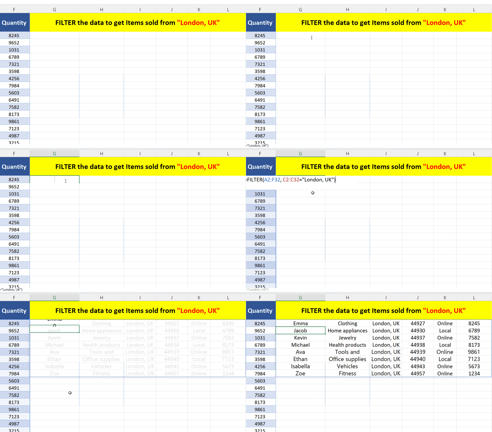
– We’ll use the following formula to get the items sold from London, UK.
=FILTER(A2:F32, C2:C32=”London, UK”)

A2:F32 represents the whole data range and C2:C32 represents the location column on which we’ll apply the criteria to get items from the dataset which are sold from London, UK.

– The obtained results are as follows above.

Note: We can avoid the above mentioned step and use this formula inside the SUMPRODUCT as shown in the next step. This is shown here just for the sake of illustrating how the FILTER function works.