How to use & sign in Excel
Microsoft Excel has a very simple method to do this by using the & Ampersand sign in formulas. Excel has many functions which are more sophisticated and can be used more dynamically to achieve the same goal. These functions are as follows;
- CONCATENATE
- TEXTJOIN
However, in this tutorial we’ll learn how to combine two cell’s values (numeric, text or alphanumeric) using the Ampersand ( & ) sign only.

Microsoft Excel allows users to format, organize and calculate data in a spreadsheet. By organizing data using Excel, data analysts and other users can make information easier to view as data is added or changed. Excel contains a large number of boxes called cells that are arranged in rows and columns. Most of the time we need to concatenate two cell’s values in order to present the data from two cells together.
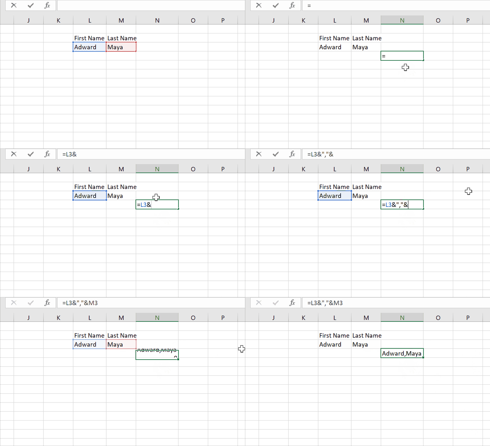
Step 1 – Select the cell and use ampersand

– Select a cell in which you wish to continue the values.
– Type = sign, select the first cell add & sign , select the second cell.
– It will concatenate the data without space.
– To add space or any other special character like comma(,) , dot(.) , space etc.
– We’ll use the following formula to join data from cells L3 and M3.
=L3& “,”&M3
By using ampersand we are now able to join two cell’s values. We added comma (,) to separate the two values. We can use any other delimiter of our own choice to join the data values from various cells. This is the most basic way to use & Ampersand in Excel. However, you can make use of this special ability of & Ampersand to your own requirements.


