
How to use Sequence in Excel
 By
SpreadCheaters
By
SpreadCheaters
In this tutorial, we’ll learn how to use this special feature of Excel effectively. Let’s understand the syntax of this function first.
Syntax of the SEQUENCE function
SEQUENCE is a dynamic array function introduced in in Excel for Microsoft 365, Excel 2021, and Excel for the web. The result of this function is a dynamic array of numbers only that spill into the specified number of rows and columns automatically.
Following is the basic syntax of the function:
SEQUENCE(rows, [columns], [start], [step])
Where:
rows
This is the number of rows to be filled. This is the mandatory parameter; without this it won’t work.
[columns]
This is the number of columns to be filled. This is an optional parameter. If you omit this, the default value of 1 will be used.
[start]
This is the starting number in the sequence. This is an optional parameter. If you omit this, the default value of 1 will be used.
[step]
This is the increment for each subsequent value in the sequence. This is an optional parameter. If you omit this, the default value of 1 will be used. It can be positive or negative.
- Use a positive step to create a sequence in ascending order.
- Use a negative step to create a sequence in descending order.
There was a time when if you had to put numbers in sequence in Excel then you had to do all the work manually. However, those days are gone now with the evolution of modern Excel, you can create a simple number series by means of Auto Fill feature. If you want to create a special sequence customized to your requirements then it is better to use the SEQUENCE function, which is specially designed for this purpose.
Step 1 – Sequence with one parameter only
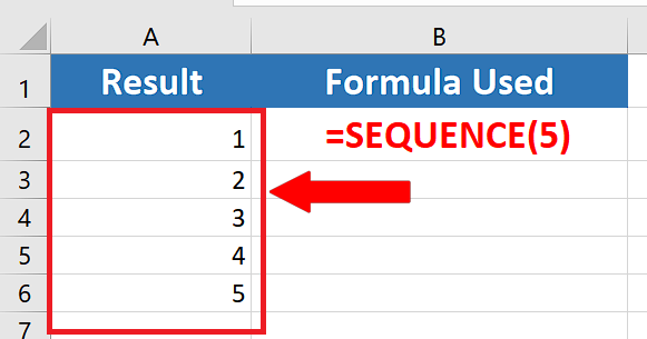
– As discussed above, this function has many variations. Let’s try the first one by using the simple formula shown below;
=SEQUENCE(5)
As we used only one parameter, i.e., the number of rows, Excel took all other parameters from default values of 1 and produced an array of 5 numbers.
Step 2 – Use Sequence to generate numbers in ascending order
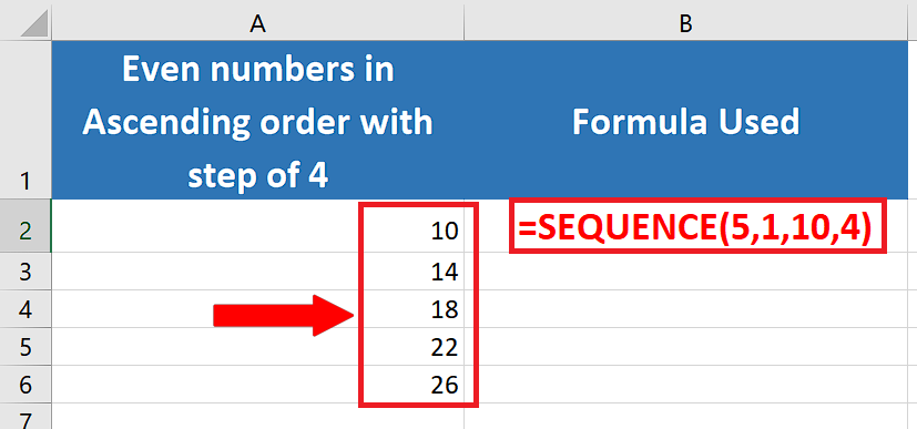
– Let’s use the following formula to generate a single column array of 5 even numbers in ascending order starting from 10 with a positive step of 4.
=SEQUENCE(5,1,10,4)
Step 3 – Use Sequence to generate numbers in descending order
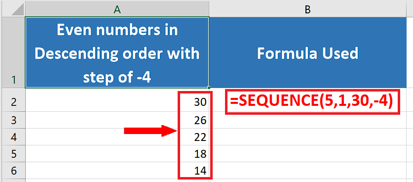
– Let’s use the following formula to generate a single column array of 5 even numbers in descending order starting from 30 with a negative step of 4.
=SEQUENCE(5,1,30,-4)
Step 4 – Generate a 2-dimensional sequence in ascending order moving horizontally
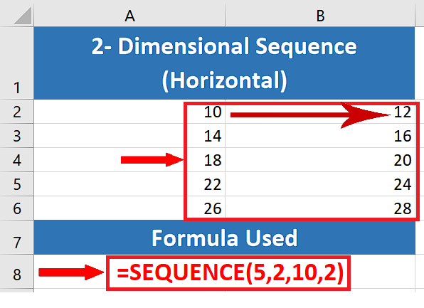
– Let’s use the following formula to generate a 2-dimensional array of 10 even numbers in ascending order starting from 10 with a positive step of 2. By default, Excel creates the array moving horizontally, i.e., the next number of the sequence will be produced in the cell available right of the first cell.
=SEQUENCE(5,2,10,2)
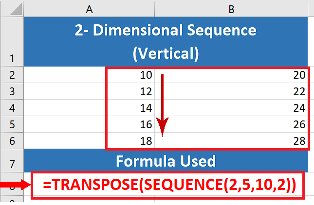
Step 5 – Generate a 2-dimensional sequence in ascending order moving vertically
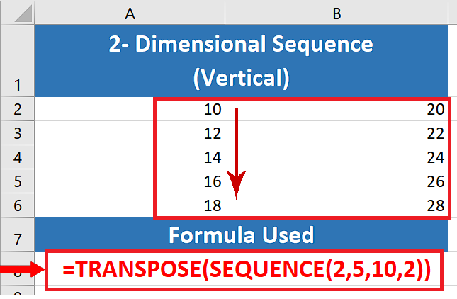
– By default, Excel creates the array moving horizontally. To create a vertically moving 2-dimensional array we’ll use TRANSPOSE before SEQUENCE. However, to nail this perfectly, you need to remember that TRANSPOSE changes the rows into columns and columns into rows. So, we need to swap the numbers of rows and columns used in the last formula to create the same number of rows and columns but in a vertical direction. The new formula is presented below;
=TRANSPOSE(SEQUENCE(2,5,10,2))
Step 6 – Generate a 2-dimensional sequence of Roman Numbers
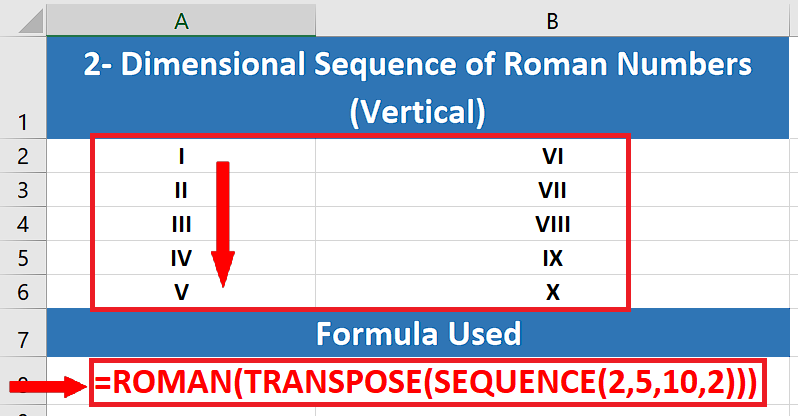
– We can use the ROMAN function in conjunction with SEQUENCE to produce a sequence of Roman Numerals as well. We’ll use the following formula;
=ROMAN(TRANSPOSE(SEQUENCE(2,5,10,2)))


