
How to use OR function in Excel
 By
SpreadCheaters
By
SpreadCheaters
Let’s first understand how the OR function works and how it evaluates the combination of criterion given to it. The syntax of the OR function is as follows;
OR(logical1,[ logical2],[ logical3],…)
The OR function can check more than one logical condition at the same time. It can combine up to 255 conditions. Each argument (logical1, logical2, etc.) must be a logical expression that can return TRUE or FALSE.
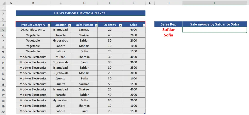
In this tutorial we’ll learn how to use the OR function in Excel to combine logical conditions to check if our data meets the criterion or not. Let’s take a look at the following sales dataset above. It has sales records of various items from various cities. We would like to create a combination of criteria to find if the sales invoice was generated by either of two specific sales reps i.e., Sofia or Safdar.
Let’s follow the steps mentioned below and get the desired results.

Excel has very powerful features for handling text, numeric and alphanumeric data as well. It also provides us with functions for making logical decisions based on a criterion. Sometimes, we need to know if some data meets a certain combination of criteria or otherwise. In this situation, we can use Excel’s logical formula OR for decision making.
Step 1 – Create the formula using OR to combine the conditions
– For our purpose, we’ll write the names of the sales reps in two different cells. In our case, we will write Safdar and Sofia in the cells H5 and H6 respectively.
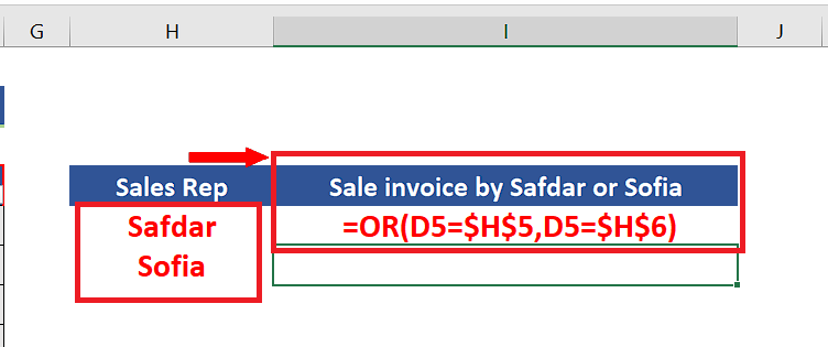
– Now write the following formula in the cell I5,
=OR(D5=$H$5,D5=$H$6)
We have used absolute references for H5 and H6 because we’ll apply the formula to the whole range of sales reps by dragging down the fill handle. We don’t want the cell references to the names of sales reps to change, therefore, we used the absolute references.
Step 2 – Implement the formula to check the criteria
– Now we’ll implement this formula by pressing enter and then extend the formula to the whole data range by dragging down the fill handle to the last row as shown above.


