How to use Not Equal <> in Excel

Excel provides a variety of operators to check various logical conditions and Not equal is also one of those operators which can be used to check whether a value is equal to another or not. In this tutorial we will learn how we can use Excel’s Not equal “<>” operator with a few very simple examples.

Example 1 – Using NOT EQUAL <> directly to compare

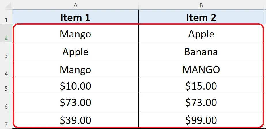
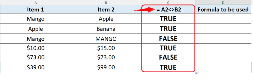
We can use the NOT EQUAL <> condition in Excel directly in any cell to compare two values and if the values are not equal to each other the result will be TRUE otherwise FALSE will be returned. We can compare the text and numbers in a similar way so let’s take an example data set and compare values in it. The data set is shown above.

Step 1 – Use <> to compare the values

• Choose a suitable cell where you wish to get the results of the comparison.
• Use the following formula in that cell and press enter key.

= A2 <> B2

• The result of the comparison will be displayed in this cell as soon as you will press the enter key as shown in the picture above.

• Just drag down the formula to implement to all rows and you will see all results of the comparison. We can see here that NOT EQUAL <> has returned TRUE in each cell where the contents of the cells are not equal to each other. This comparison is case-insensitive. That’s why we got a FALSE while comparing Mango and MANGO. The comparison has also worked with numbers alike. So this operator can be used to compare data including text and numbers in a similar way.

Example 2 – Using NOT EQUAL <> with IF function

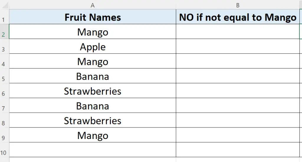
As the NOT EQUAL to is a logical operator so it can be used inside any formula that can test logical conditions. For example if we wish to compare two texts and want to produce a meaningful result then we can use this operator inside an IF function. Let’s take a look at this data set, where we wish to find out if a fruit is a Mango or otherwise.

To use the “IF” function properly we need to understand the syntax of the formula and what parameters it requires to work. So let’s see the structure of the formula first and then we’ll apply this to a data set to see the formula in action.

Structure of IF Function:

The structure of the IF function in Excel is fairly simple and easy to comprehend. The generic formula of an IF Function is given below;

=IF(Logical_Test_Condition, Result_if_true, Result_if_false)

This function requires the following three parameters, which are explained below one by one.

• Logical_Test_Condition:

The first parameter is the logical test condition which will be evaluated by the formula. When constructing a test condition we can use the following logical operators to evaluate a logical scenario;

• = (equal to)
• > (greater than)
• >= (greater than or equal to) 
• < (less than)
• <= (less than or equal to)
• <> (not equal to)

• Result_if_true:

The formula evaluates the logical condition and if the condition is found correct (true) then this value will be chosen to appear as a result.

• Result_if_false:

This is the value which will be chosen as a result, when the test condition is found incorrect (false) after being evaluated in the formula.

Let’s implement the formula following the below mentioned steps;

Step 1 – Use NOT EQUAL <> inside IF

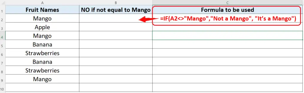
• Choose a suitable cell, which in our case is in the next column B.
• Use the following formula to check if a fruit’s name is Mango or otherwise. As shown in the figure above.

=IF(A2<>”Mango”,”Not a Mango”, “It’s a Mango”)

Step 2 – Implement the formula to get results

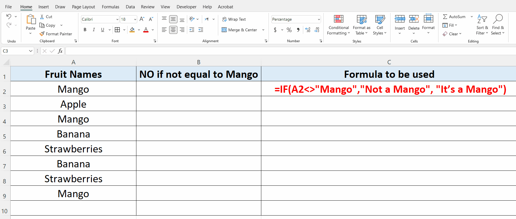
• The formula is very simple, it checks if the value in A2 is not equal to Mango then the result will be Not a Mango and if the value in A2 is equal to Mango then the result will be It’s a Mango. So let’s implement the formula and then drag it down till the last row of data set to get results just like shown in the figure above.

So in this way we can use the NOT EQUAL <> operator inside a simple formula to create a logical condition that can help us to make further necessary decisions.