
How to use Match & Sum together in Excel
 By
SpreadCheaters
By
SpreadCheaters
In such cases we use a very special combination of three of Excel’s most used formulas to create a special look up formula. The functions that we’ll use are as follows;
- MATCH
- INDEX
- SUM
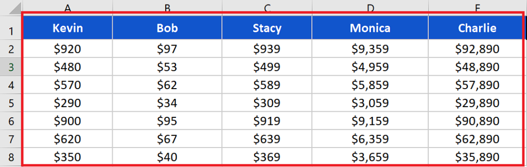
Let’s take an example data set of a grocery store and try to create and implement a special formula to find the sum of the sales made by any employee.
While working with big data sets like sales reports of big companies we often need to find a simpler way to see the performance of an employee based upon the total sales any of them has made. In such situations we need a special way to look up the data set to find out the sum of the sales made by some specific employee.
Step 1 – Create and implement the formula

– We want to create a generic formula to calculate the total sales made by an employee. The calculations will be based upon the name of the employee. So the formula that we’ll use is going to be:
=SUM(INDEX(A2:E8,0,MATCH(B11,A1:E1,0)))
Breakdown of the formula
- The formula we used was;
=SUM(INDEX(A2:E8,0,MATCH(B11,A1:E1,0)))
- The formula has three functions in it; MATCH, INDEX & SUM.
- MATCH(B11, A1:E1,0):
It looks up the value contained within cell B11 (which is obtained by a data validation list, containing the names of all employees) inside the range A1:E1 (which are the names of the employees) and returns a position as a number if a match is found. In our example it will first return 1 in case of Kevin and then 2 when we selected Bob.
- INDEX(A2:E8, 0, 1):
The first argument is the range where to look for indexing which is A2:E8.
The second argument is the heart of the whole formula, setting this row_number to zero, we force the Index function to return the whole column whose index is being returned by the match function as the third argument.
So it takes the column index number as the third argument and returns the array {920; 480; 570; 290; 900; 620; 350} to the argument of the SUM function
- The SUM function takes the array and returns the SUM in the cell and that’s how we get our desired result by using these three functions together.


