How to use INDEX MATCH across multiple sheets in Microsoft Excel

In this tutorial we will learn how to use the INDEX & MATCH functions across multiple sheets in Microsoft Excel. To use the INDEX & MATCH functions between multiple sheets in Excel, you can simply specify the sheet name followed by an exclamation mark (!) before the cell range or array reference in the formula. Then, use the MATCH function to specify the lookup criteria. By combining these two functions, you can perform lookups across multiple sheets in Excel.

We have a dataset above that displays the marks obtained by five students in five different subjects in Sheet3.Our objective is to extract the marks obtained by student 3 and place them in a separate sheet i.e.Sheet4.

INDEX MATCH is a powerful combination of two functions in Microsoft Excel. The INDEX MATCH formula can be used to retrieve a specific value from a large dataset based on criteria such as a name, date, or unique identifier. The INDEX function returns the value of a cell in a specified row and column of an array or range, while the MATCH function returns the position of a specified value within an array or range.

Step 1 – Select a Blank Cell

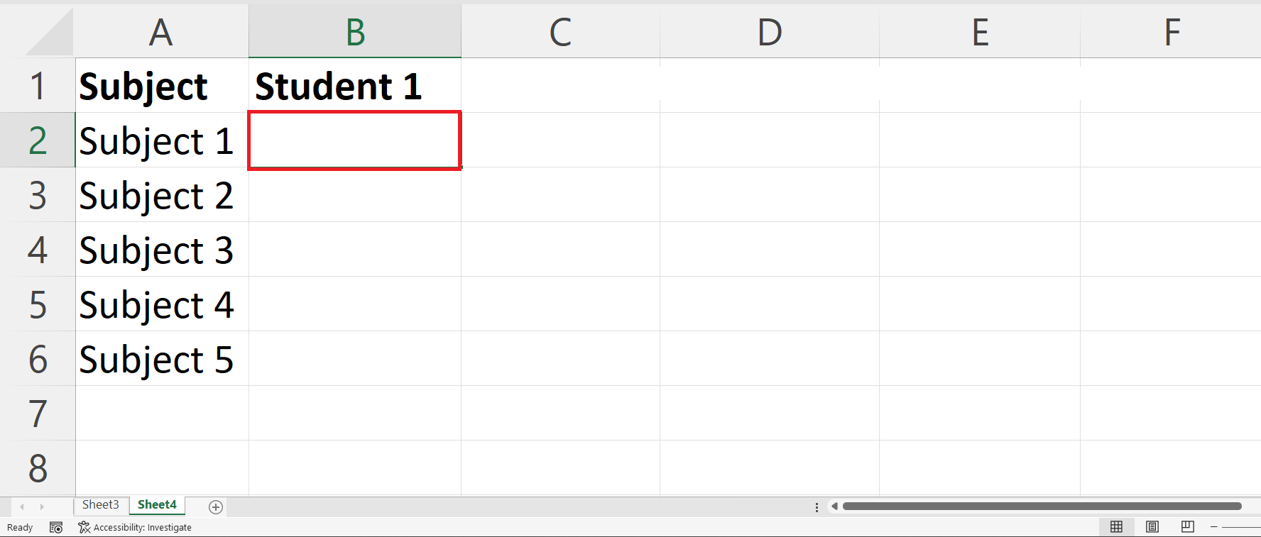
– Select a blank cell in a new sheet i.e. Sheet4 in which you want to extract the data.

Step 2 – Place an Equals Sign

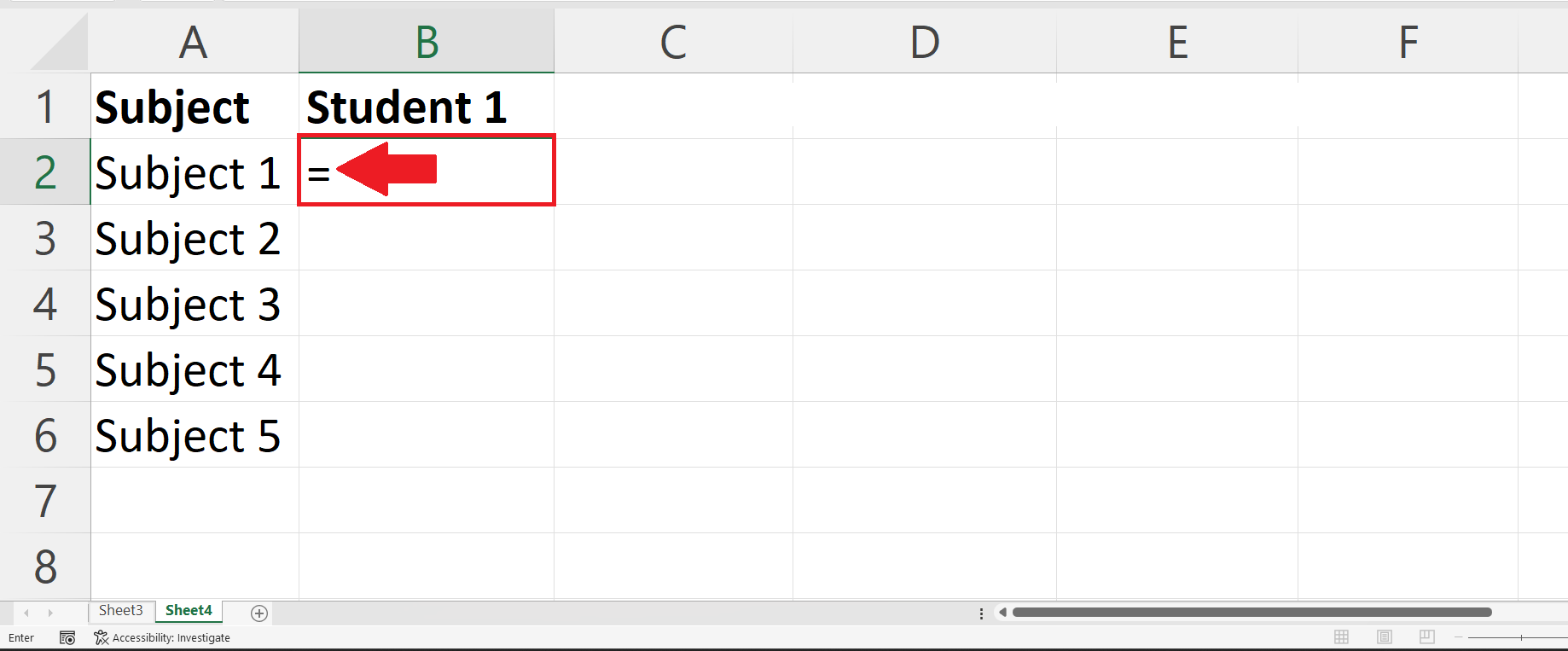
– Place an Equals Sign in the targeted blank cell.

Step 3 – Use the INDEX MATCH Functions

– Use a combination of  INDEX MATCH functions to extract the data from the data range in another sheet.
– The syntax for the combined function will be:  
     
         INDEX(Sheet3!A1:F6,MATCH(Sheet4!A2,Sheet3!A1:A6,0),MATCH(Sheet4!B1,Sheet3!A1:F1,0))

– We enter the sheet name and an Exclamation mark ( ! ) before each range to reference a range from another sheet.

Step 4 – Press the Enter Key

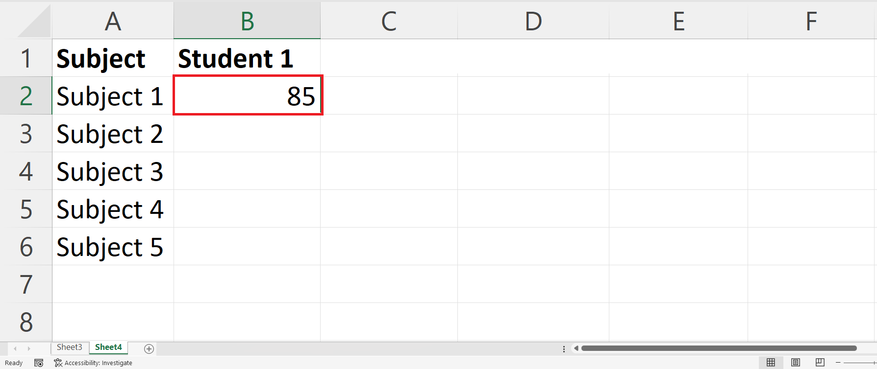
– Press the Enter key to extract the data in Sheet 4.

Step 5 – Use Autofill to Extract Data for Each Subject

– Use the Autofill feature to extract data for each subject in the adjacent cells.

Understanding the Components of Combined Function 

  INDEX(Sheet3!A1:F6,MATCH(Sheet4!A2,Sheet3!A1:A6,0),MATCH(Sheet4!B1,Sheet3!A1:F1,0)) 

We will break down the function inside out. The INDEX function accepts three arguments,i.e. The range of the data, row number and the column number.

• The third argument of INDEX function i.e. MATCH(Sheet4!B1,Sheet3!A1:F1  returns the column number of the value within an array or a range of cells. Inside the MATCH function the first argument SHEET4!C1 is the cell containing the lookup value,the Second argument Sheet3!A1:F1 is the reference of the range containing the lookup value and the last argument i.e. 0 is optional and specifies the type of match to be performed – exact match or approximate match i.e. 1 , 0 , -1.

• The second argument of INDEX function i.e.MATCH(Sheet4!A2,Sheet3!A1:A6,0) returns the row number of the value within an array or a range of cells.Inside this MATCH function the first argument SHEET4!B2 is the cell containing the lookup value, the Second argument Sheet3!A1:A6 is the reference of the range containing the lookup value and the last argument i.e. 0 is optional and specifies the type of match to be performed – exact match or approximate match i.e. 1 , 0 , -1.

• The first argument of the INDEX function i.e.Sheet3!A1:F6 is the range of the data from which you are extracting the value.