How to use IF with MATCH function in Excel

In this tutorial, we’ll learn how to use IF with the MATCH function in Excel. First of all we’ll understand the syntax of both functions and then we’ll use an example to see how a combination of both functions can be used.

Structure of IF Function:

The structure of the IF function in Excel is fairly simple and easy to comprehend. The generic formula of an IF Function is given below;

=IF(Logical_Test_Condition, Result_if_true, Result_if_false)

This function requires the following three parameters, which are explained below one by one.

Logical_Test_Condition

The first parameter is the logical test condition which will be evaluated by the formula. When constructing a test condition we can use the following logical operators to evaluate a logical scenario;

• = (equal to)
• > (greater than)
• >= (greater than or equal to)
• < (less than)
• <= (less than or equal to)
• <> (not equal to)

Result_if_true:

The formula evaluates the logical condition and if the condition is found correct (true) then this value will be chosen to appear as a result.

Result_if_false:

This is the value which will be chosen as a result, when the test condition is found incorrect (false) after being evaluated in the formula.

Now let’s see what is the syntax of MATCH and what parameters it requires to work.

Syntax of MATCH

It is very important to remember that the MATCH function will return a numeric value which will correspond to the position index of the lookup value in the given array. It will not return TRUE or FALSE. In case the lookup value is not found in the given array the result will be #N/A (value not available) error.

The syntax of this function is as follows;

=MATCH(lookup_value, lookup_array, [match_type])

 lookup_value:

It is the value that will be searched.

lookup_array:

It is the range of data in which the lookup value will be searched

[match_type]:

This is an optional parameter which will tell Excel how to search the array. The MATCH function has three options here. 

1 = This will find the largest value that is less than or equal to the lookup_value. Lookup array must be placed in ascending order, otherwise you will get incorrect results.

0 = With this option used, the MATCH function finds the first value equal to the lookup value. Lookup array can be in any order.

-1 = MATCH will find the smallest value that is greater than or equal to the lookup_value. Lookup array must be placed in descending order, otherwise you will get incorrect results.

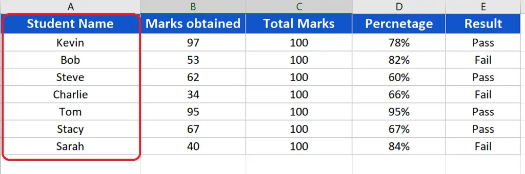
Now let’s see how we can utilize the power of both functions in a combined way. We have a data set with the names and marks data of some students and we wish to find out if a student’s name exists in the data set or not. To achieve this we’ll use the combination of IF and MATCH functions.

While we are operating with data which includes text information along with numeric data then it is a very common requirement to use logical conditions to sort, find and analyse the data. Microsoft Excel provides us with a lot of functions to process and analyse the data in a logical way. Sometimes we have to use a combination of two or more functions to get our required results.

One such combination of functions is IF along with MATCH.

Step 1 – Create an appropriate formula

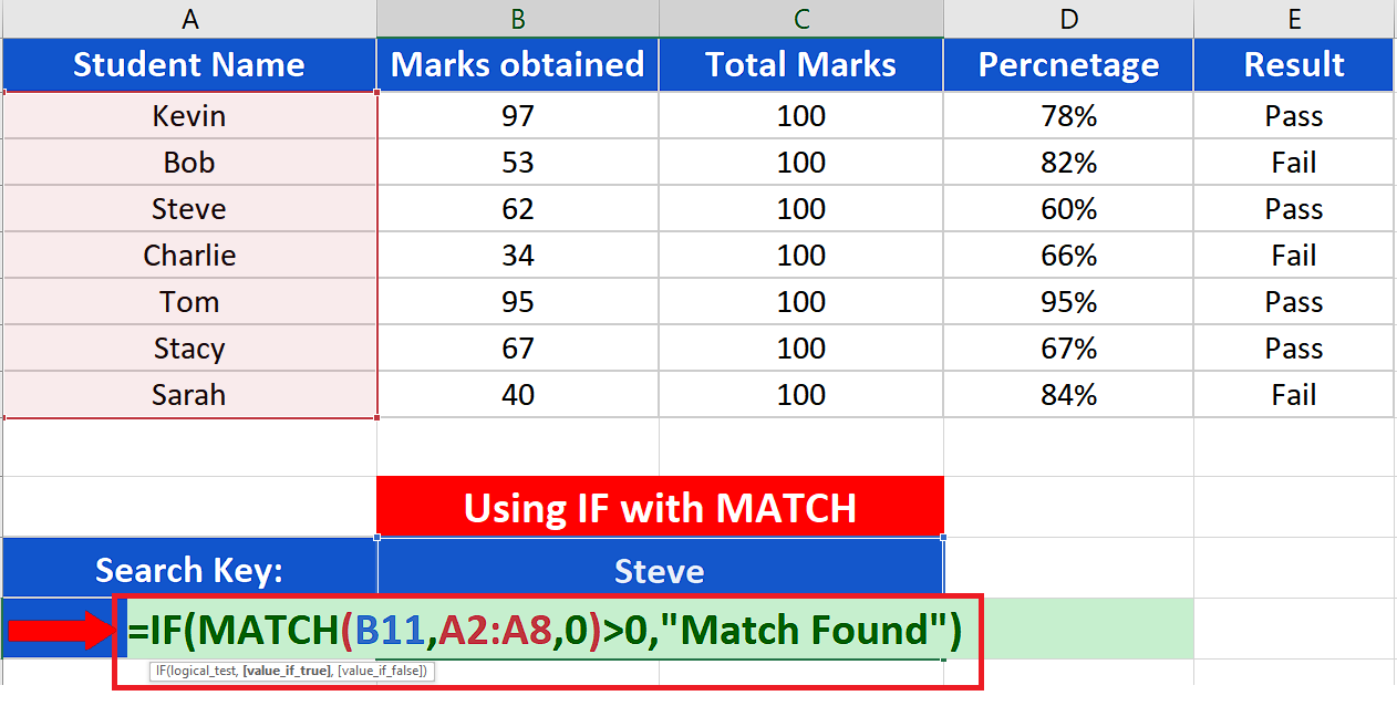
– Choose a cell where you wish to get the result of the search and write down this formula;

=IF(MATCH(B11,A2:A8,0)>0, “Match found”)

If the match is not found the MATCH function will automatically return an #N/A (value not available) error.

Step 2 – Implement the formula

– Now it’s time to implement the formula. So after writing the formula in an appropriate cell press Enter. The results of the formula will be shown in the cell in the above picture.

We can use more complex combinations of the formulas to look up for the marks of the respective student whose name is present in the given array of data. However, for that we’ll have to use INDEX along with IF & MATCH functions as well which is beyond the scope of this topic.

Breakdown of the formula used:

We used MATCH inside the IF function, so let’s understand what MATCH is doing first. The MATCH function searches for the lookup value, which is the name of the student in cell B11, in the given array of data i.e. A2:A8. If the name is found inside the given array then the numeric position index of the name will be returned. However, we wish to display a meaningful result when the name is found so we enclosed the output of MATCH inside an IF. We will check if the MATCH function returns a numeric value greater than ZERO, then it means a match if found so we’ll display “Match Found” instead of the position index. If no match is found then the MATCH function will automatically display #N/A, value not available error.