
How to use IF function between two number in Microsoft Excel
 By
SpreadCheaters
By
SpreadCheaters
In this tutorial we will learn how to use the IF function in Microsoft Excel. The IF function in Microsoft Excel is a powerful tool that allows you to make logical comparisons between values and take actions based on the result. In its simplest form, the IF function tests a condition and returns one value if the condition is true and another value if it is false.
Microsoft Excel is a spreadsheet program widely used by businesses, organizations, and individuals to manage, analyze, and present data. Excel provides a flexible and intuitive interface for working with data. It allows you to organize data in cells and worksheets, perform calculations using formulas and functions, and create charts, tables, and pivot tables to visualize and analyze data. Additionally, Excel provides a number of advanced features such as conditional formatting, data validation, and macros for automating repetitive tasks.
Step 1 – Select a Blank Cell
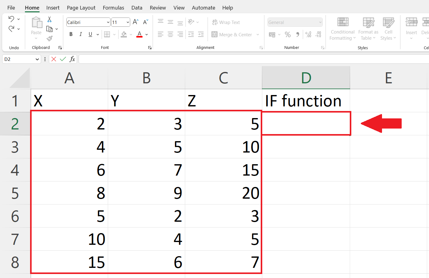
– Select a blank cell where you want to get the output.
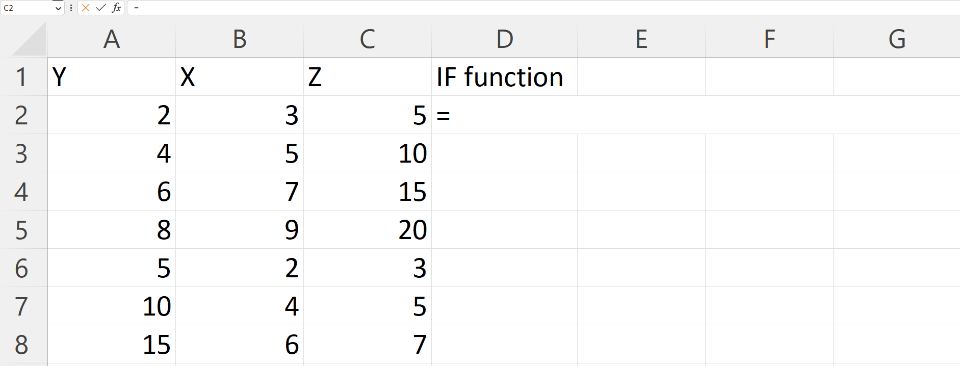
Step 2 – Place an Equals Sign
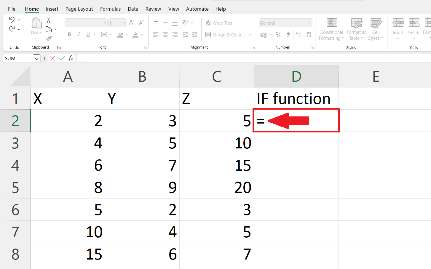
– Place an equals sign(=) in the targeted cell.
Step 3 – Use the IF function
– Enter the If function next to the equals sign. The IF function tests a condition and returns one value if the condition is true and another value if the condition is false. For using IF function between two number the syntax will be :
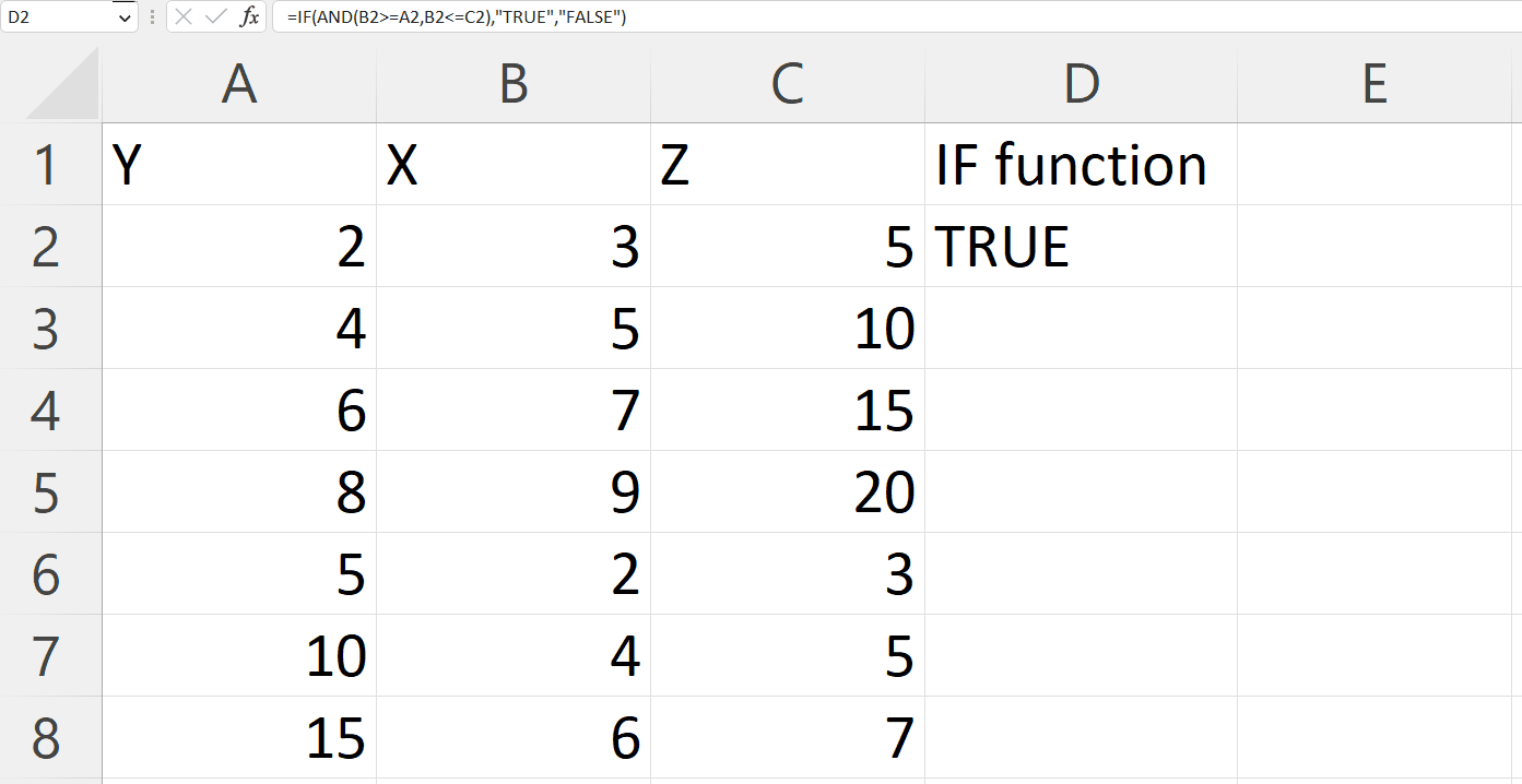
=IF(AND(X>=Y,X<=Z),”True”,”False”)
– X is the number to be tested and Y to Z is the range in which X is to be tested.
– Where the IF function will check if X is greater than equal to Y and X is smaller than equal to Z.
– If both arguments are satisfied than function will return “True” and if not than “False”
Step 4 – Press Enter Key
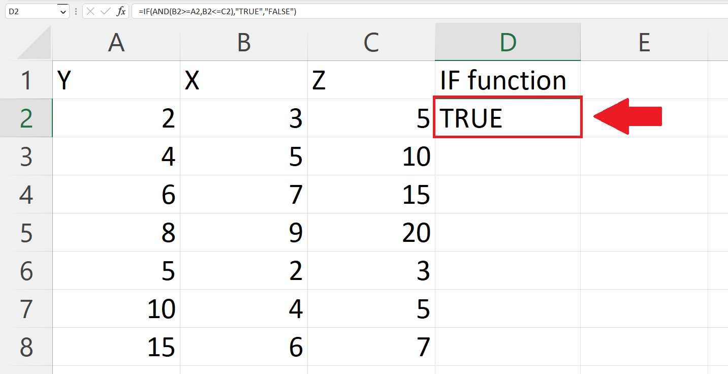
– Press the Enter key to get the result.
Step 5 – Apply the IF function on each row

– Use the “Handle Select” and “Drag and Drop” method to apply the function on each row.


