
How to use filter function with multiple criteria in Excel
 By
SpreadCheaters
By
SpreadCheaters
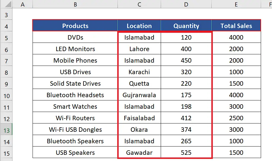
In today’s tutorial we’ll learn how to use the FILTER function in Excel with multiple criteria. Let’s look at the dataset given above. It contains the sales data of various products from various locations.
Follow along the steps mentioned below to learn how to apply two types of filters (AND, OR) using the FILTER function with multiple criteria using on the dataset in Excel. Let’s learn the syntax of FILTER and see what parameters are required to use this formula properly.
Syntax of FILTER
The syntax of the FILTER function is as follows,
=FILTER(array, include, [if_empty])
array:
This is the range (B4:E15 in our case) from which we’ll filter the values based upon the include criteria.
include:
This is the Boolean array created through the criteria applied on the range data. In our case this will be C4:C15 for filtering location and D4:D15 for filtering the quantity sold.
[if_empty]:
The value to return if all values in the included array are empty (filter returns nothing). This is an optional parameter and we’ll not use it in our example.

The Filter function in Microsoft Excel allows you to extract and display only the relevant data from a large data set based on certain criteria. This can help to simplify and organize data, making it easier to analyze and draw insights. The good thing about using the filter function is that the original data remains unchanged, and you can remove the filter at any time.
Step 1 – Choose cells for dynamic criteria
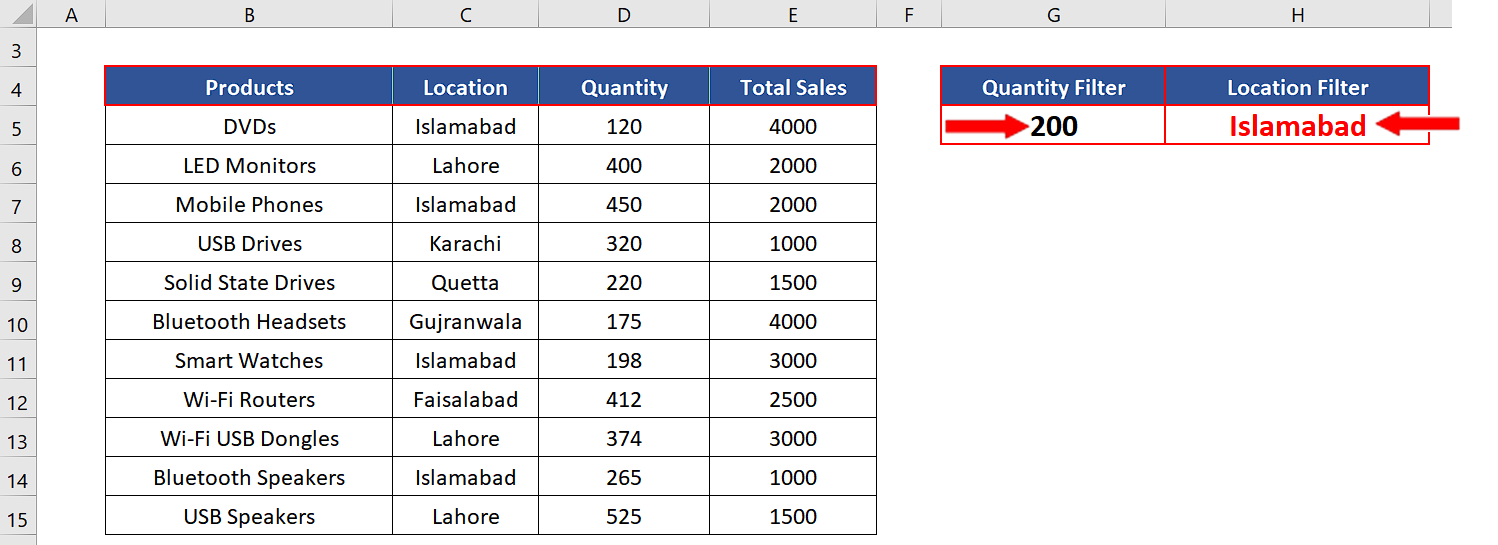
– Select two cells outside the data table.
– Give it a suitable name. For our example, we’ll use “Quantity Filter and Location Filter”.
– Choose an appropriate value which will be checked inside the criteria range. We’ll choose 200 for Quantity and Islamabad for Location as the filtering, as shown above.
Step 2 – Create the filter formula with Quantity AND Location Criteria
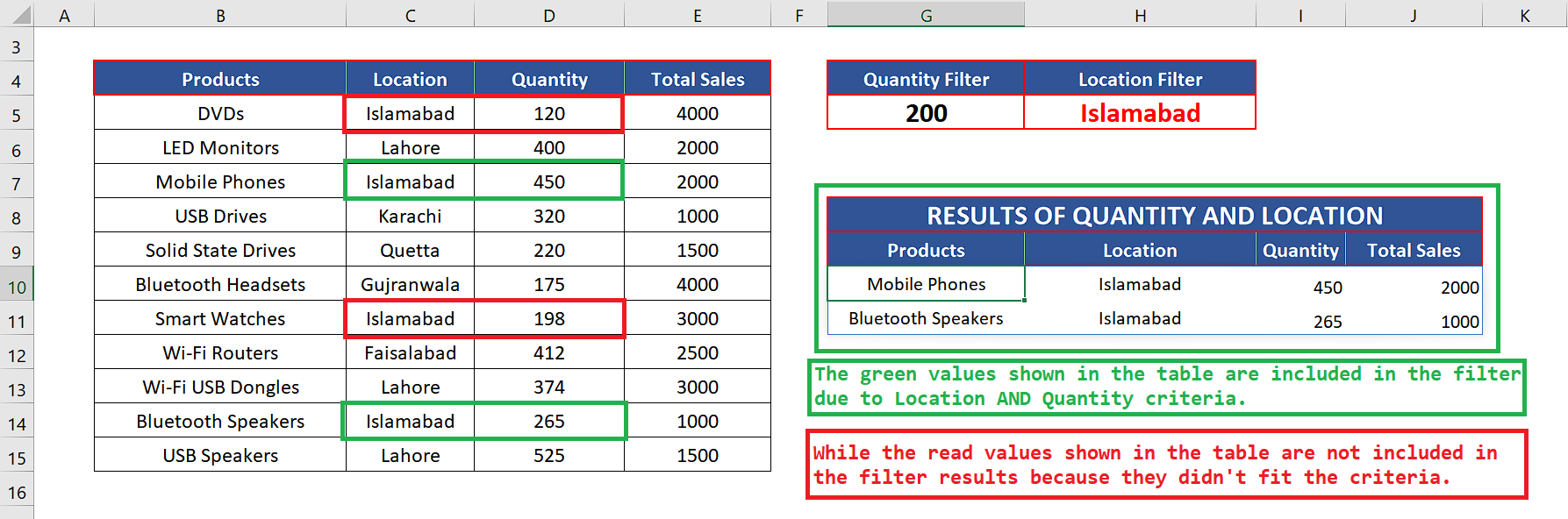
– We’ll use the following formula for filtering with AND condition for Quantity and Location, as shown below.
=FILTER(B5:E15,(C5:C15=H5)*(D5:D15>=G5))
The * sign between the two criteria enclosed in parenthesis creates an AND condition. So, we’ll get only those results which satisfy both conditions i.e., Quantity greater or equal to 200 AND Location is Islamabad only.
Step 3 – Change the AND criteria dynamically
– We have set up the FILTER function in such a way that when we change the values in the cells G5 (represents quantity) and H5 (represents location), the FILTER criteria will be updated and new results will be populated automatically as shown above.
Step 4 – Create the filter formula with Quantity OR Location Criteria
– We’ll use the following formula for filtering with AND condition for Quantity and Location, as shown below.
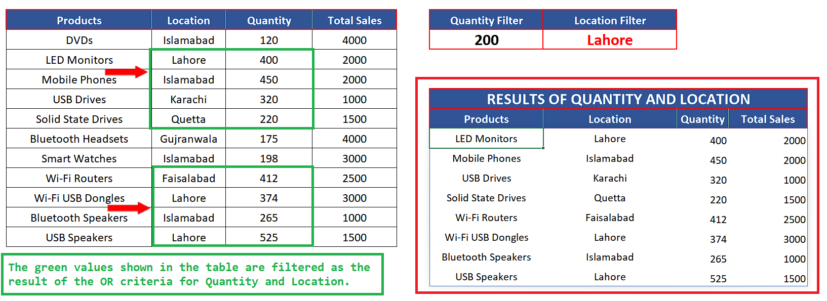
=FILTER(B5:E15,(C5:C15=H5)+(D5:D15>=G5))
The + sign between the two criteria enclosed in parenthesis creates an OR condition. So, we’ll get only those results which satisfy both conditions i.e., Quantity greater or equal to 200 OR Location is Islamabad only.
Step 5 – Change the OR criteria dynamically
– We can change the results in the similar way we did in Step 3 by changing any value either in the quantity filter or Location filter as shown above.


