
How to use Ctrl + T in Excel
 By
SpreadCheaters
By
SpreadCheaters
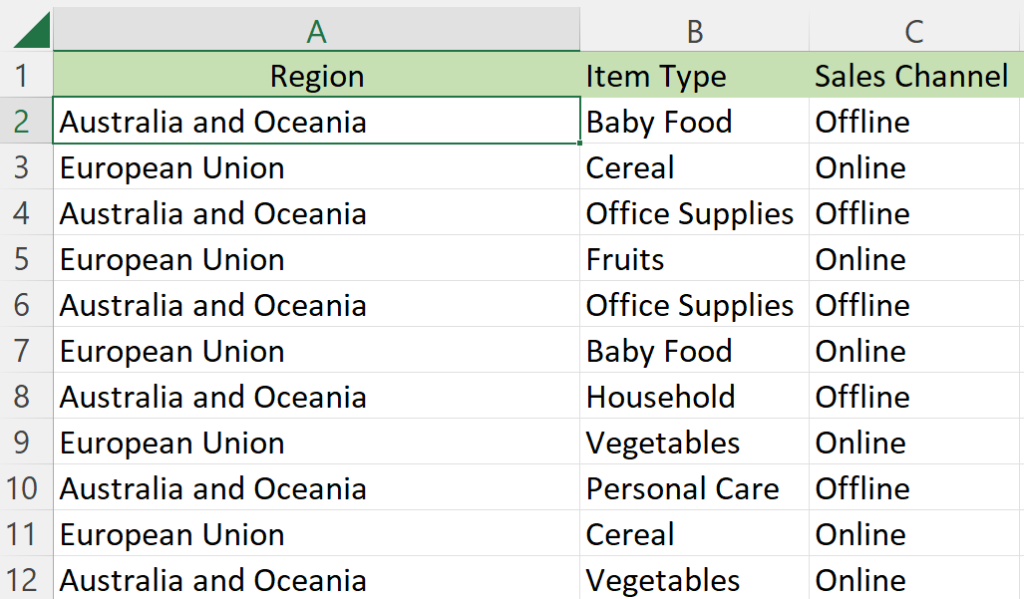
In today’s tutorial, we’re going to learn how to use Ctrl + T to insert a table in our already existing range data. So, here we have a dataset containing some information about region, item type and sales channel of the sellers. Consider the following dataset above as an example for learning how to use this shortcut key.
We’re going to convert this range data into a table by using this shortcut. Follow these steps below to use this shortcut key:
A table in Microsoft Excel is a set of data organized in a grid of rows and columns, and it is designed to be used for analyzing and manipulating the data efficiently. Tables provide several benefits, such as sorting, filtering, and formatting options, dynamic calculations using structured references, and easy expansion when new data is added.
Following are benefits of tables:
– Structured references: Allows you to refer to table data using simple, intuitive, and dynamic references that automatically adjust as the table grows or changes.
– Auto-expanding: As you add new data to the table, it automatically expands to include the new data, without the need to manually adjust the range of the data source.
– Sorting and filtering: Allows you to quickly sort and filter the data in the table based on various criteria, making it easier to analyze and manipulate the data.
– Formatting: You can apply a predefined table style to the entire table with a single click, giving it a professional and organized look.
Step 1 – Using Ctrl + T shortcut key to convert range to table

– Select any cell from the range of cells e.g., B8.
– Then, press Ctrl + T.
– After that, a small pop-up box will appear.
– Select the “OK” option.
– Now, your data will be converted to a table.
Step 2 – Inserting new table by using Ctrl + T shortcut key
– Select any blank cell.
– Then, press Ctrl + T.
– After that, a small pop-up box will appear.
– Select the “OK” option.
– Now, your table is created and you can adjust its columns and rows according to your requirement.


