How to use Countif to count the non blank rows in Excel

The best way to understand how countif works is to first understand the structure of the function and the parameters it requires.

Structure of COUNTIF

The standard syntax of countif function in excel is shown below;

= COUNTIF(range,criteria)

• range (where to look in for something)

A range can be a single column with multiple rows or it could consist of multiple columns and multiple rows. For example “A1:B10”. This will tell the formula to search through two columns A & B till the 10th row.

• criteria (what to look for)

Criteria will be a special logical test which will depend upon the situation and the nature of values that we are looking for. In our example we are looking for all non-blank cells so we will use a special logical condition in the formula which will tell Excel to count only those cells which are not blank.

Implementing the Formula on an Actual Data Set

Let’s take an example data set and find out the number of non empty or non-blank cells in it. So let’s consider the data set shown below;

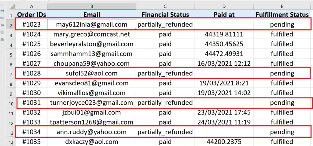
We can see in the example data set that a blank entry in the “Paid at” column shows that the task fulfilment status is pending. So it means if we want to know how many tasks have been completed then this can be achieved by counting the non-blank cells in that particular column.

Let’s see how we can use Excel’s built-in formulas to find a solution to our problem by following these steps;

When we are working with data sets to analyse them in Excel, often there is a requirement to count those cells which are not empty. Excel provides some very easy ways to find out the number of non-blank cells within a specific range. In this tutorial we will learn how we can use Excel’s built-in “COUNTIF” function to calculate the number of cells which are not empty. 

Step 1 – Implement the formula in a suitable cell:

– Choose a suitable cell where you wish to implement the formula.

– Use the following formula in that cell and press enter key.

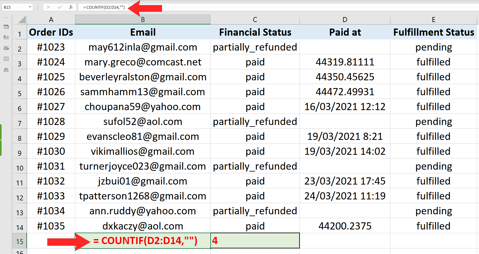
=COUNTIF(D2:D14,”<>”&””)

– The desired result will be displayed in this cell as soon as you will press the enter key as shown in the picture above;

So by using COUNTIF with a special condition to count the blank rows in column D we can find out that only 9 tasks are completed in the tasks lists.

Breakdown of the Logical Condition used inside the formula

We used the formula =COUNTIF(D2:D14,”<>”&””). Let’s see how we told Excel where to look and what to look for. 

• The first parameter D2:D14 tells Excel that the data range in which we are going to look for something is in column D and from row 2 to row 14 only.
• The second parameter was “<>”&””. The “<>” represents a logical condition Not Equal to and “” is a special character which represents a “BLANK”. So when we use this combination in the condition parameter it tells Excel to look for a cell that is not blank. When Excel finds a non-blank cell with anything in it. The counter is increased. Our data set had nine non-blank cells in that range so the result was 9 as desired.