
How to use a formula to determine which cells to format
 By
SpreadCheaters
By
SpreadCheaters
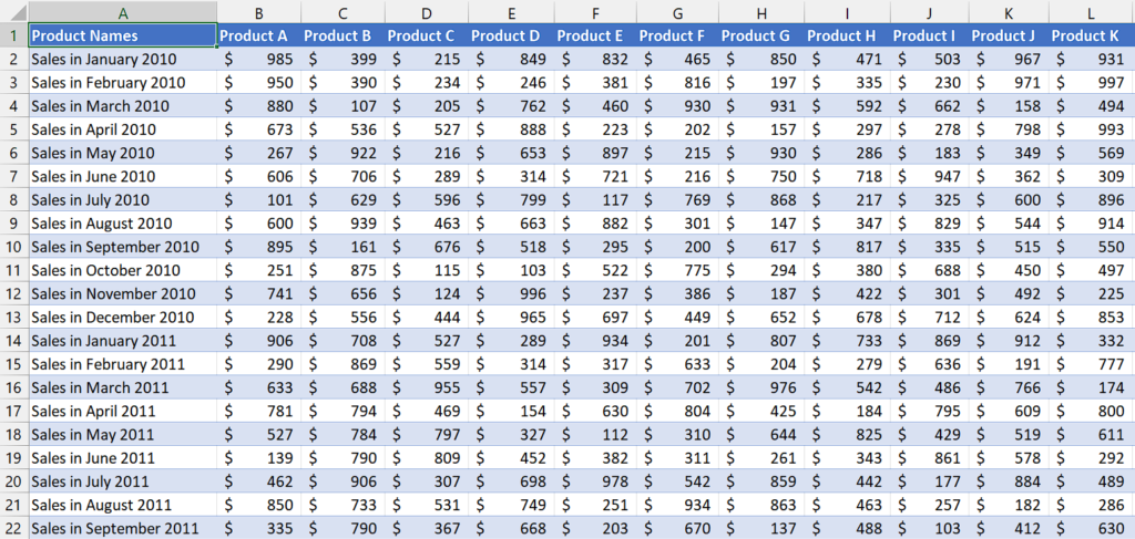
In this scenario, we have sales data for 26 products spanning a period of 5 years. The objective is to understand how to apply a formula to determine the formatting of specific cells based on this data.
Formatting cells based on formulas can help you quickly identify patterns, trends, or outliers in your data. By applying specific formatting rules, you can emphasize important information or draw attention to specific values, making it easier to interpret and analyze the data.
Step 1 – Select the cell range
– Select the cell range in which you want to format the cells based on the formula.
– We will apply conditional formatting to this cell range.
Step 2 – Add a rule for conditional formatting
– Go to the “Home” tab in the Excel ribbon.
– Click on the “Conditional Formatting” button, located in the “Styles” group. A drop-down menu will appear.
– From the drop-down menu, select “New Rule.” The “New Formatting Rule” dialog box will open.
Step 3 – Use a formula to format cells
– After the “New Formatting Rule” dialogue box has opened, click on the last option which is “Use a formula to determine which cells to format”.
– Then, enter the formula that you wish to use to format cells.
– For instance, we used this formula,
=ISNUMBER(SEARCH(“2012”,$A1))
ISNUMBER: It is a function in Excel that checks whether a value is a number. In this case, it will be used to evaluate the result of the SEARCH function.
SEARCH(“2012”,$A1): This function searches for the text “2012” within the value of cell $A1. It returns the starting position of the text if found, and an error value if not found.
$A1: It represents a cell reference in Excel. In this case, it refers to column A and the current row number (1 if applied to the first row).
– Basically, we will use this formula as a condition in conditional formatting to format cells containing the text “2012”.
Step 4 – Set format for specific cells
– Click on the “Format” button and then select the formatting that you wish to do with the specific cells such as changing the fill color, background color and etc.
Step 5 – Apply Formatting
– After you’ve followed the above steps, click on the “OK” button and conditional formatting will be applied.


