
How to unhide multiple rows in Excel
 By
SpreadCheaters
By
SpreadCheaters
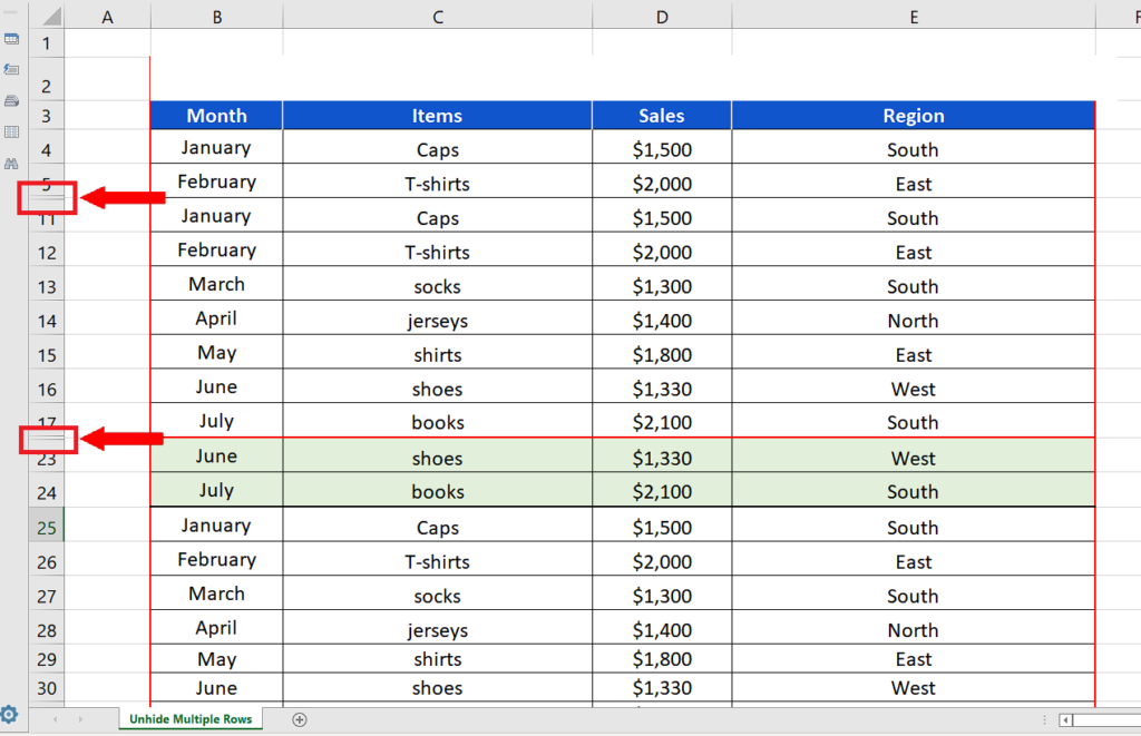
In this tutorial we’ll learn how to unhide multiple rows in Excel by following these simple steps. The dataset given above has multiple hidden rows i.e., row 6 to row 10 and row 18 to row 22.

Excel being a powerful tool for visualization and manipulation of data, provides very efficient and simple methods to present the data. It also provides tools to hide unnecessary data while still keeping the data in the spreadsheet and vice versa.
Step 1 – Select rows before and after the hidden rows or select the whole sheet
– The key to unhide multiple rows is to select the row right before and after the hidden rows. If your sheet has hidden rows at multiple places then just select the whole sheet by clicking on the arrow in the top right corner of the spreadsheet as shown above.
Step 2 – Use the shortcut key CTRL + SHIFT + 9 or use Context Menu’s Unhide option
– The method to unhide multiple rows is very simple, after selecting the appropriate rows just use the shortcut key CTRL + SHIFT + 9 (number key) or right click and use the Unhide option from the context menu.
– Both options will unhide all hidden rows inside the selected rows.


