How to unhide data in Excel

In Excel, “hiding” data means to make it temporarily invisible or not visible to the viewer. “Unhiding” data in Excel means reversing the process of hiding and making the data visible again. Unhiding data can increase transparency and accountability. Unhiding data can foster innovation by making information available to researchers and developers. Once the hidden data is unhidden, it will be visible again to anyone viewing the spreadsheet. While working in Excel, we can only hide and unhide rows and columns.

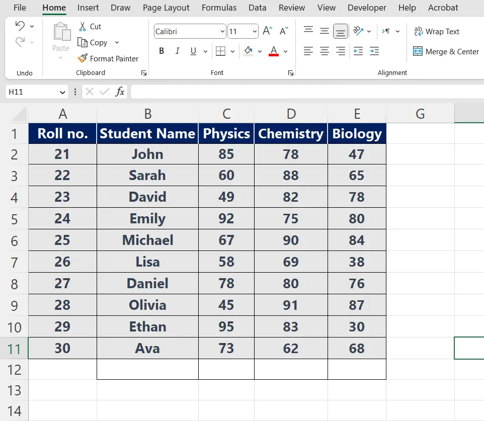
In this tutorial, we will learn, how to unhide data in Excel. The following data shows the roll numbers of the students and their names and their marks in physics, chemistry, and biology. In the following dataset a column in which the marks of students in the subject Mathematics are already hidden, let’s learn how to unhide it. 

Method 1 – Unhiding column through the Home tab

There are 2 methods to unhide columns in Excel. In this method, we are going to unhide columns through the home tab. Consider the following steps to learn how to unhide columns through the Home tab in Excel. 

Step 1 – Select the columns

• Select the columns to the left and right of the hidden columns.

Step 2 – Go to the home tab

• Go to the home tab.
• Go to Format in the cells group.

Step 3 – Click on Format.

• After clicking on Format, a dropdown menu will open.
• Click on Hide & Unhide option, which is available under visibility.

Step 4 – Click on Unhide columns.

• When you will click on Hide & Unhide, a dropdown menu will appear.
• Select any option from that menu, as per our requirement we will select unhide columns.
• When you will click on Unhide columns, the columns will be unhidden. 

Method 2 – Unhiding column through the context menu

In this method, we are going to unhide columns using the context menu. This method is simpler and easier than the method discussed above. Follow the given steps to learn how to unhide data using the context menu.

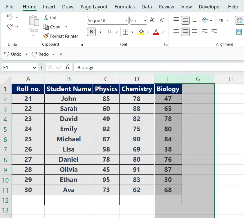
Step 1 – Select the adjacent columns

• Select the columns left and right to the hidden column.
• When you right-click, a context menu will appear.

Step 2 – Select unhide

• From that context menu, select unhide.
• The hidden columns will be unhidden.

Conclusion:

In this step-by-step guide, we learned that we can unhide columns of data that were initially hidden from the sheet. It is worth mentioning here that these methods are applicable to both rows and columns equally. Therefore, using the same methods we can also unhide the hidden rows in our sheet.