How to turn rows into columns in Excel

Microsoft Excel is a very useful tool for manipulating data whether it is numeric or text. In this tutorial we’ll learn how to change the way to visualise data by changing the data in rows to columns.

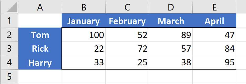
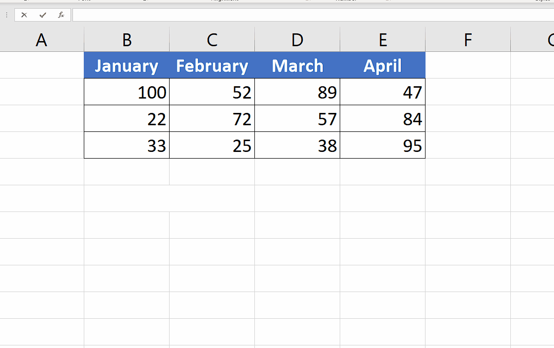
Excel provides very simple methods for achieving this goal. Let’s explore the methods one by one by applying both methods to the following simple dataset.

Method 1 Use Transpose from Paste Menu Options

Step 1 – Select and copy all relevant data

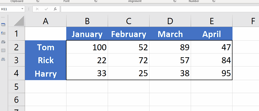
• Select all relevant data and then press CTRL+C to copy the data.

Step 2 – Paste the data using Transpose option from Main Paste Menu or Context Menu Options

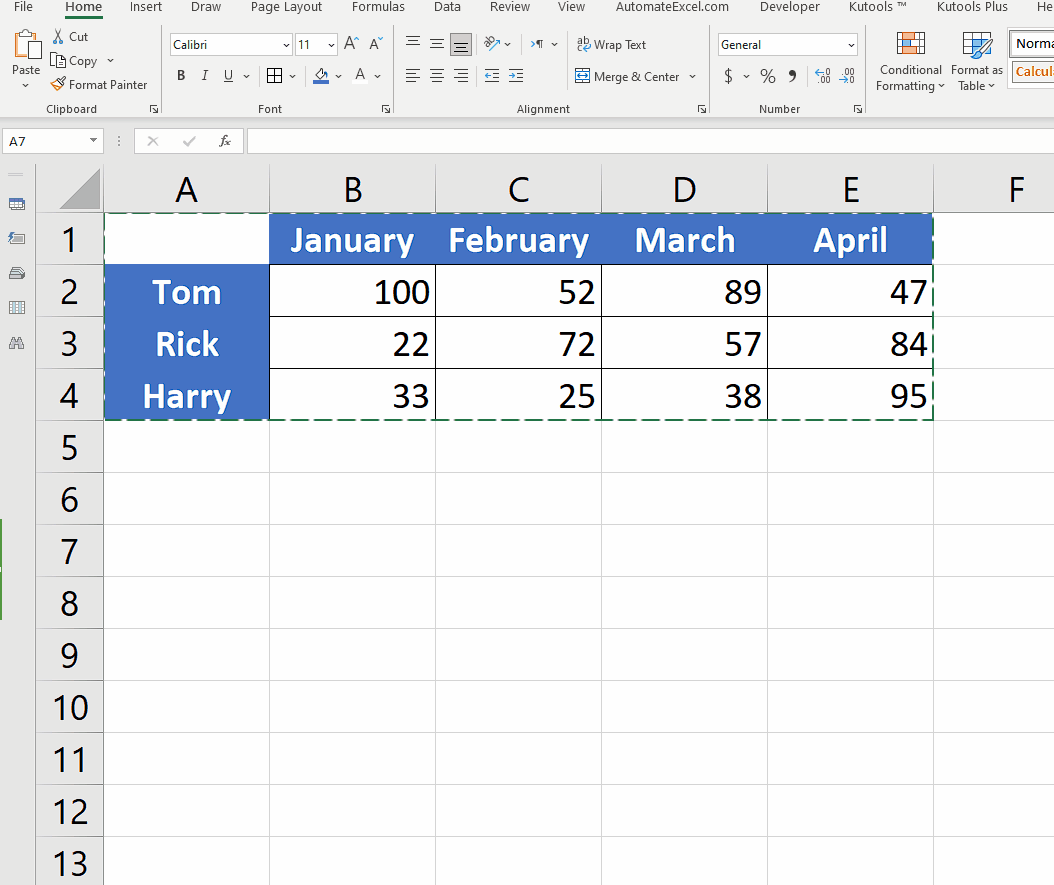
• Now click on the cell where you wish to place the new data. Right click in that cell and it will open the context menu. 
• In this menu go to Paste options: and click on icon. It will convert the data from rows into columns and paste it starting from the selected cell.
• The same goal can be achieved by going to Paste options in the Clipboard group on the main menu and then choosing the same icon as before.

Method 2 Use Transpose Function

Excel has a built-in function to transpose an array. It takes only one argument i.e. the data range as an array and changes the rows into columns. Let’s implement it on the following dataset.

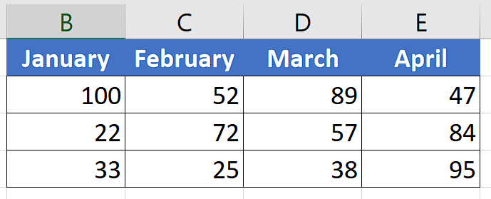
Step 1 – Select the cell and implement the Transpose formula

• Select the appropriate cell and implement the following very simple formula in it. This will change all the rows into columns and columns into rows as shown below.

=TRANSPOSE(B1:E4)