How to turn off the scientific notation in Microsoft Excel

Scientific notation is a way to represent very large or very small numbers in Excel. In Excel, scientific notation is denoted by using the letter “E” to represent “x10^”. Excel uses scientific notation to display large or small numbers that are difficult to display in standard number format. When a number is too large or too small to display in a standard format, Excel automatically converts it to scientific notation so that it can be displayed in a compact and readable form.

In this tutorial, we will learn how to turn off scientific notation in Microsoft Excel. We can convert the scientific notation to standard number format in Excel using the Format Cells option, which allows you to change the formatting of the cell to display the number as a simple number. Additionally, function as the TRIM function or the CONCATENATE function can be utilized. Also, a  simple method involves adding an apostrophe before the number to force Excel to treat it as a text value rather than a numeric value, which will prevent it from being automatically converted to scientific notation.

Method 1: Changing the Format of the Cell

Step 1 – Select the Cells and Right Click

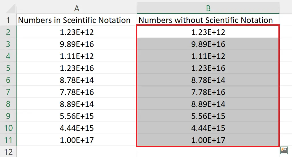
• Select the cells containing the numbers in scientific notations.
• Right-click on the selected cells containing the numbers in scientific notation.
• The context menu will appear.

Step 2 – Click on the Format Cells Option

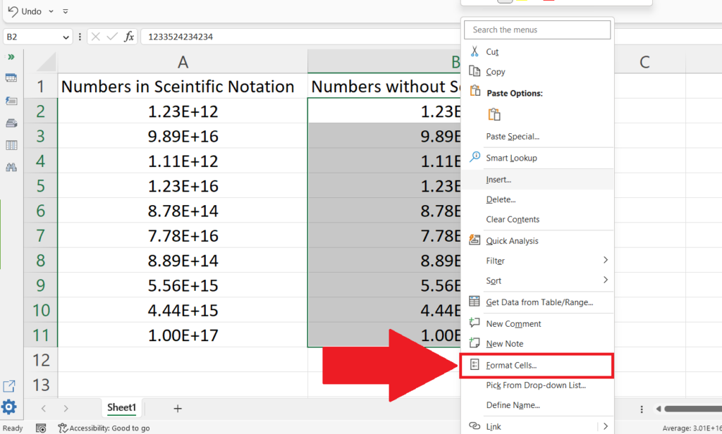
• Click on the Format Cells option in the context menu.

Step 3 – Select Number as the Format

• Select Number as the format of the cell.

Step 4 – Click on OK

• Click on OK in the Format Cells dialog box.
• The number will be changed to standard form.

Method 2: Using the TRIM Function

Step 1 – Select a Blank Cell and Place an Equals Sign

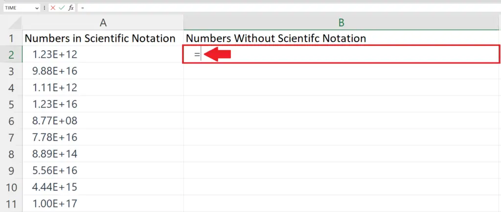
• Select a  blank cell and place an equals sign in the cell where you want to place the number in the standard form.

Step 2 – Enter the TRIM Function

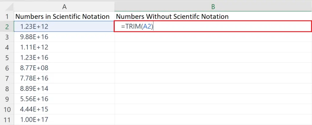
• Enter the TRIM function.
• The syntax of the TRIM function will be: 

                                 TRIM(A2)

• Where A2 is the cell containing the number in scientific notation.

Step 3 – Press the Enter Key

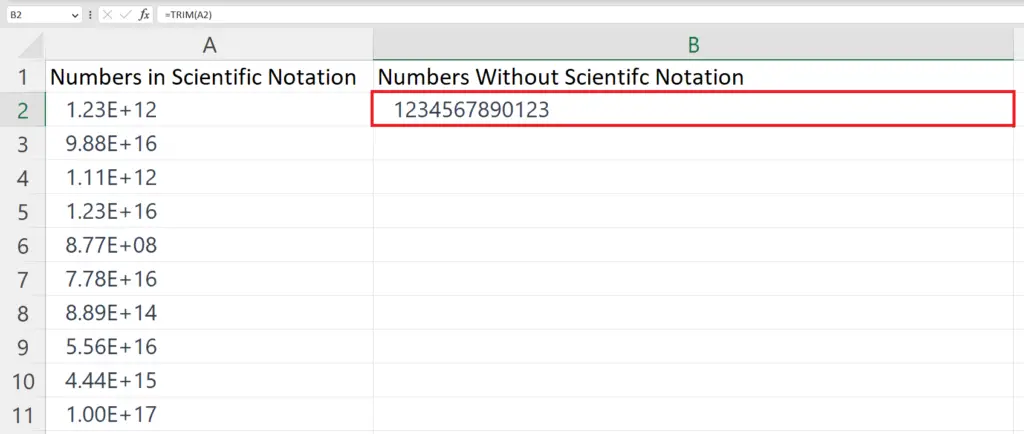
• Press the Enter key to remove the scientific notation.

Step 4 – Use the Autofill to Apply the Function on Each Number

• Use Autofill to apply the function on each number.

Method 3: Using the CONCATENATE Function

Step 1 – Select a Blank Cell and Place an Equals Sign

• Select a  blank cell and place an equals sign in the cell where you want to place the number in the standard form.

Step 2 – Enter the CONCATENATE Function

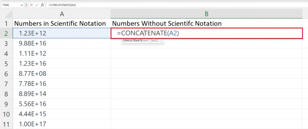
• Enter the CONCATENATE function.
• The syntax of the CONCATENATE function will be: 

                                CONCATENATE(A2)

• Where A2 is the cell containing the number in scientific notation.

Step 3 – Press the Enter Key

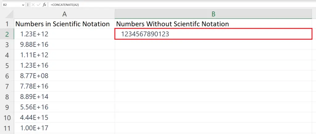
• Press the Enter key to remove the scientific notation.

Step 4 – Use the Autofill to Apply the Function on Each Number

• Use Autofill to apply the function on each number.

Method 4: Placing an Apostrophe at the Start of the Number

Step 1 – Double Click on the Cell

• Double-click on the cell containing the number in scientific notation.

Step 2 – Place an Apostrophe 

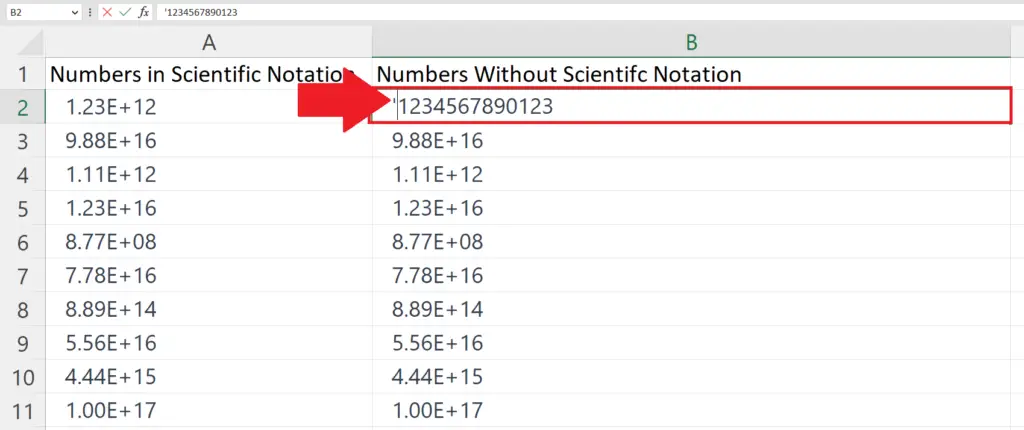
• Place an Apostrophe ( ‘ ) at the start of the number.
• The number will be converted into the standard form.

Step 3 – Use the Autofill to Place an Apostrophe at the Start of Each Cell

• Use the Autofill to Place an Apostrophe at the Start of Each Cell