
How to truncate text in Microsoft Excel
 By
SpreadCheaters
By
SpreadCheaters
In this tutorial we will learn how to truncate text in Microsoft Excel. Truncating text in Microsoft Excel refers to the process of limiting the number of characters displayed from a longer text string. This is useful when you want to display only a portion of the text, or when you have limited space to display the full text and want to avoid text overflow. In Excel, you can truncate text using the LEFT, RIGHT, and MID functions.
Microsoft Excel is a spreadsheet software developed by Microsoft Corporation. It is widely used for data analysis, organization, and manipulation of various types of data. Excel features a user-friendly interface, formula-based calculation, charting and graphing tools, and the ability to create macros for automating repetitive tasks. It supports various file formats including .xlsx, .xls, and .csv and can be used on multiple platforms, including Windows, macOS, and mobile devices. With its powerful tools and versatility, Excel is a crucial tool for individuals, businesses, and organizations to manage, analyze, and visualize their data.
Method 1 : Truncate Text using LEFT function
Step 1 – Select a blank cell
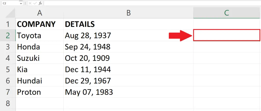
- Select the targeted cell where you want to truncate the text.
Step 2 – Place an equals sign
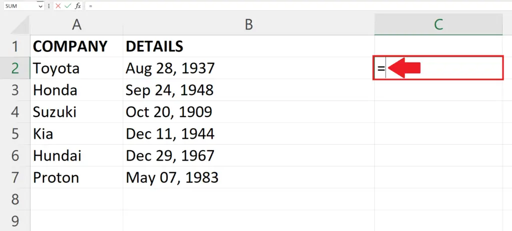
- Place an equals sign (=) in the targeted cell.
Step 3 – Use the LEFT function

- Enter the LEFT function next to the equals sign (=).The LEFT function returns the first “n” characters from the beginning of the text string.
LEFT(B2,n)
- Where “n” is the number of characters you want to truncate and B2 is the cell address containing the text.
Step 4 – Press the Enter key
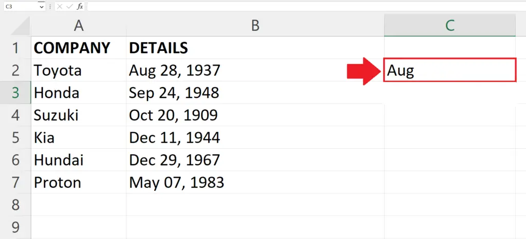
- Press the Enter key to truncate the text.
Step 5 – Apply the LEFT function to each row
- Use the “handle select” and “drag and drop” method to apply the LEFT function on each row.
Method 2: Truncate text using MID function
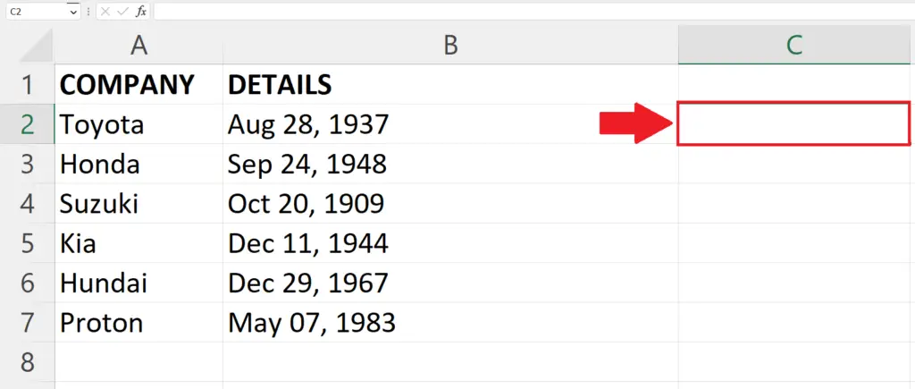
Step 1 – Select a blank cell

- Select the targeted cell where you want to truncate the text.
Step 2 – Place an equals sign
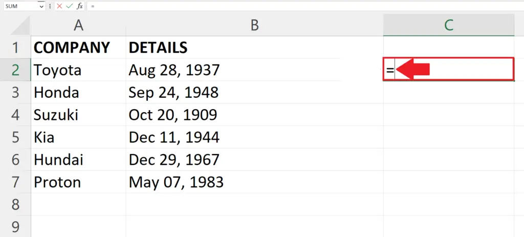
- Place an equals sign (=) in the targeted cell.
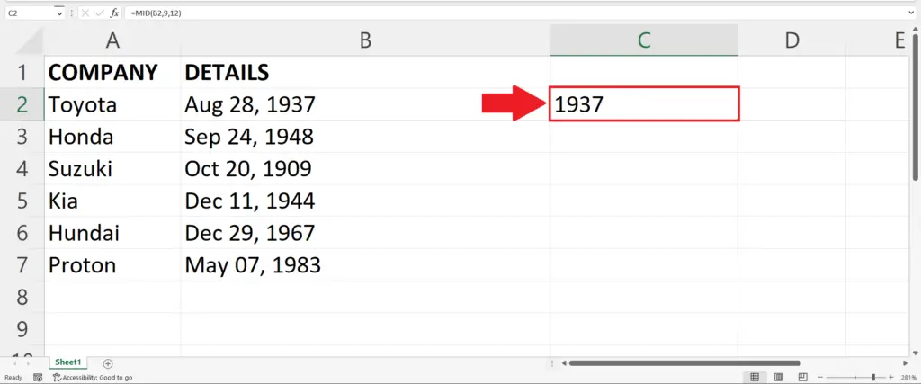
Step 3 – Use the MID function
- Enter the MID function next to the equals sign (=).The MID function returns the first “n” characters from the beginning of the text string.
MID(B2,n)
- Where “n” is the number of characters you want to truncate and B2 is the cell address containing the text.
Step 4 – Press the Enter key
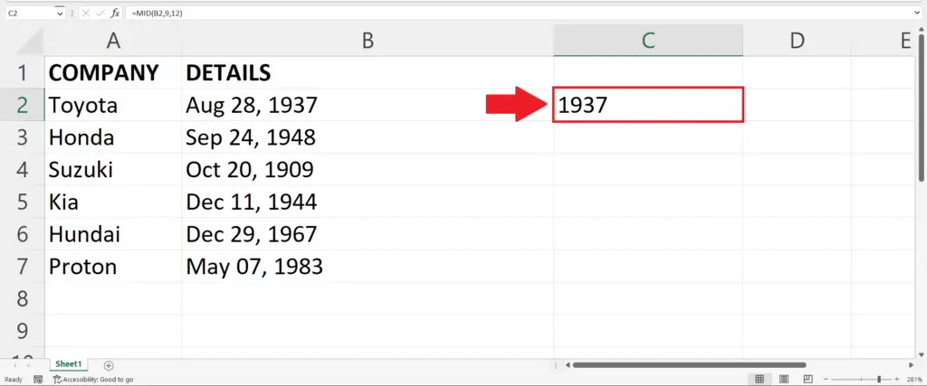
- Press the Enter key to truncate the text.
Step 5 – Apply the MID function to all rows

- Use the “handle select” and “drag and drop” method to apply the MID function on each cell.
Method 3: Truncate text using RIGHT function
Step 1 – Select a blank cell
- Select the targeted cell where you want to truncate the text.
Step 2 – Place an equals sign

- Place an equals sign (=) in the targeted cell.
Step 3 – Use the Right function
- Enter the Right function next to the equals sign (=).The RIGHT function returns the first “n” characters from the beginning of the text string.
RIGHT(B2,n)
- Where “n” is the number of characters you want to truncate and B2 is the cell address containing the text.
Step 4 – Press the Enter key
- Press the Enter key to truncate the text.
Step 5 – Apply the Right function to all rows
- Use the “handle select” and “drag and drop” method to apply the Right function on each cell.
Method 4 : Using Text to Column Option
Step 1 – Select a blank cell
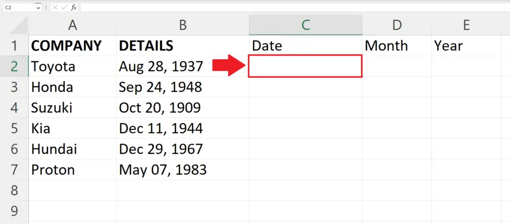
- Select a blank cell from where the text should start.
Step 2 – Select the Column
- Select the column containing the text which you want to truncate.
Step 3 – Go to Data
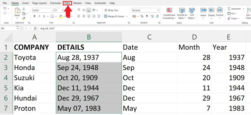
- Go to the Data in the menu bar.
Step 4 – Click on the Text to Columns option
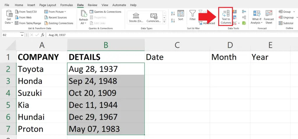
- Click on the Text to Column option in the Data tools section.
Step 5 – Click on the Delimited option
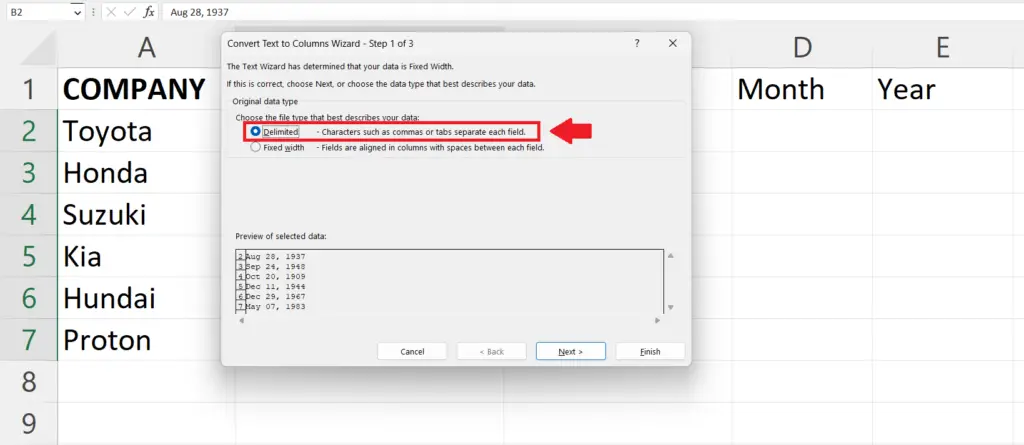
- Click on the Delimited option in the Convert text to columns wizard, Step 1.
Step 6 – Click on Next
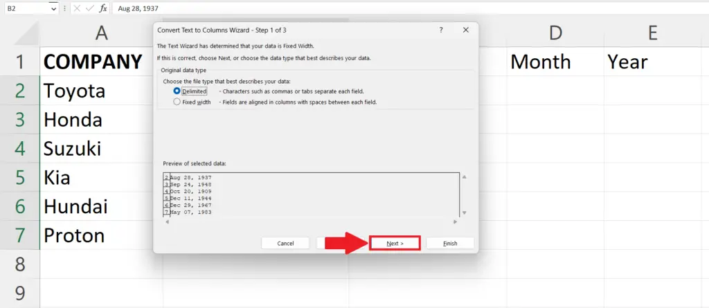
- After clicking on Delimited, option click on Next.
Step 7 – Select Delimiters
- Select the Delimiters in the convert text to columns wizard, Step 2.
Step 8 – Enter the address of targeted cells
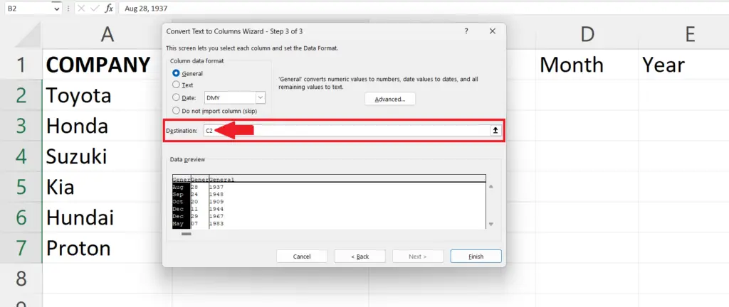
- Enter the address of the targeted cell in the Destination option in the convert text to columns wizard, Step 3.
Step 9 – Click on Finish
- Click on FInish to get the results


