How to take screenshots in an Excel Sheet

Screenshots are a great way to capture data and information in Excel, allowing you to quickly share it with others. There are different ways to take screenshots in Excel, and in this tutorial, we’ll discuss the various methods you can use.

Here we have a dataset, in this dataset, there are Car brands and the Number of Cars Sold. We will now learn two different methods of how to take Screenshots in excel but first let’s take a look at the Dataset above.

Method – 1 Using Excel camera tool.

Step – 1 Locate the camera tool

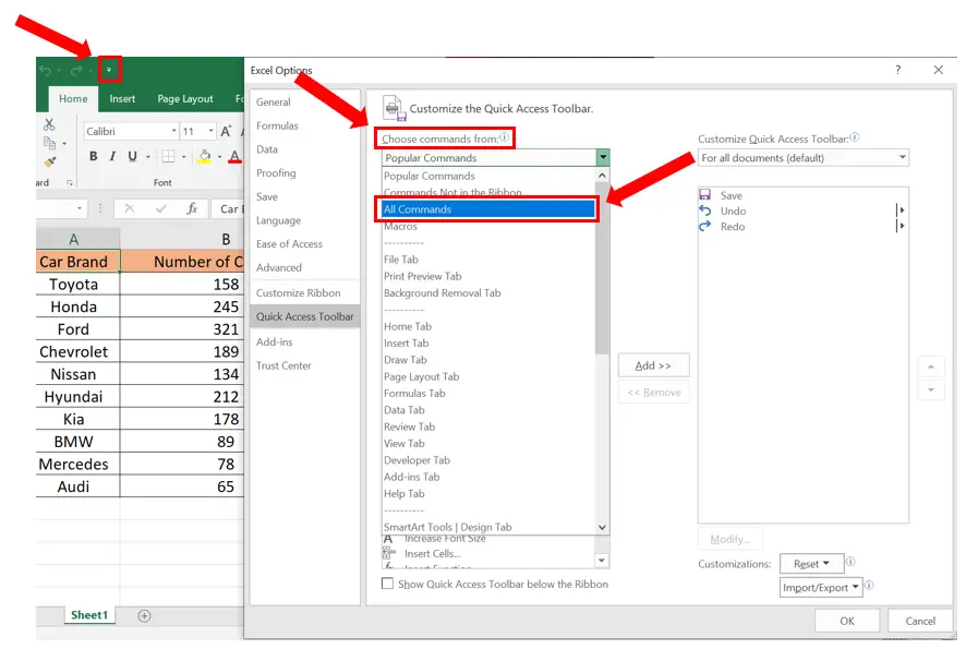
• Go to the Quick Access Toolbar at the top of the Excel sheet and click on the More Commands option.
• This will reveal a dialog box containing the Choose Command From dropdown menu.
• Click on the dropdown menu and choose All Commands.

Step – 2 Add the camera tool.

• In the <Separator> menu find the Camera Tool.
• Click Add then click Ok.
• This will add the camera tool in the Quick Access Toolbar.

Step – 3 Take a Screenshot.

• Select the table you want to take a screenshot of.
• Select the camera tool and then click on the table you have chosen.
• The screen will be taken.

Method – 2 Using the Snipping Tool.

Step – 1 Selecting the tool.

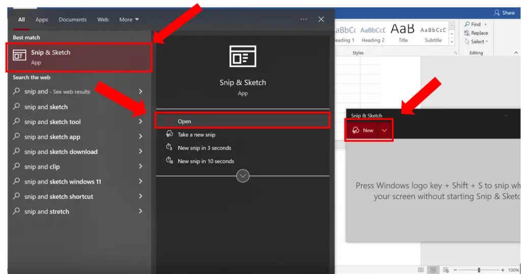
• Go to the Search button and search Snip & Sketch.
• Open the App and click on New.
• Alternatively, you may use the shortcut key Windows Button + SHIFT + S to open up the snipping tool.

Step – 2 Take a Screenshot.

• Drag the cursor over the area you want to take a screenshot of.
• The screenshot will be taken.
• You can also click on the print screen button on your keyboard to take a screenshot.
• Then save them in the location of your choice.