
How to SUMIF multiple columns in Excel
 By
SpreadCheaters
By
SpreadCheaters

Here we have a dataset that contains data about Employee, Department, Salary and Bonuses of three months. In this tutorial, we will learn how to find the total bonus of the Sales Department by following the steps below. Let’s have a look at the dataset above first.

Excel is a powerful tool for managing and analyzing data. One of the most common tasks in Excel is calculating totals based on specific criteria. For example, you might want to calculate the total sales for a particular product or the total expenses for a specific department. The SUMIF function in Excel makes it easy to do this by allowing you to sum values based on a specific condition or criteria.
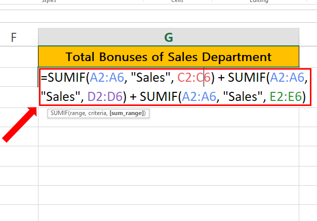
Step 1 – Type the formula.
– Click on the cell where you want to find the sum.
– Syntax of the formula:
=SUMIF(range, criteria, [sum_range]) + SUMIF(range, criteria, [sum_range]) + SUMIF(range, criteria, [sum_range])
Range: Cells that you want to evaluate for the criteria. In this formula, A2:A6 is the range that contains the fruits.
Criteria: The criteria that you want to apply. In this formula, “Sales” is the criteria you want to apply.
[sum_range]: Cells that you want to sum. In this formula, C2:C6, D2:D6, and E2:E6 are the ranges that contain the sales figures that you want to sum.
– In our case Formula will be:
=SUMIF(A2:A6, “Sales”, C2:C6) + SUMIF(A2:A6, “Sales”, D2:D6) + SUMIF(A2:A6, “Sales”, E2:E6)
Step 2 – Apply the formula.

– After typing in the formula click enter.
– Sum of all the Bonuses from all the months where the department is “Sales” will be calculated as shown above.
Breakdown of the formula
We have used the following formula
=SUMIF(A2:A6, “Sales”, C2:C6) + SUMIF(A2:A6, “Sales”, D2:D6) + SUMIF(A2:A6, “Sales”, E2:E6)
This formula uses SUMIF to perform a conditional SUM on the respective cells from the ranges C2:C6, D2:D6, E2:E6 when the Department name is Sales in the Search Range which is A2:A6.The plus sign + used in between the SUMIF formulas tells Excel to add up all results together.


