
How to sum values based on criteria in another column in Excel
 By
SpreadCheaters
By
SpreadCheaters
You can watch a video tutorial here.
One of the great things about Excel is the ease with which complex and simple mathematical operations can be done. Excel has several tools and functions that can be used to aggregate numbers. Adding a range of numbers is quite straightforward but there are functions that you can use to add numbers based on criteria. Assume you have a list of orders for different items and you want to find out how many units of each item are required.

In Excel, this can be done using the SUMIF() function.
1. SUMIF() function: this adds numbers based on a criteria
a. Syntax: SUMIF(criteria range, criteria, sum_range)
i. criteria range: the range to be evaluated by the criteria
ii. criteria: the criteria
iii. sum_range: the range to be added. This is optional and needs to be given only if it is different from the criteria range
Step 1 – Create the formula
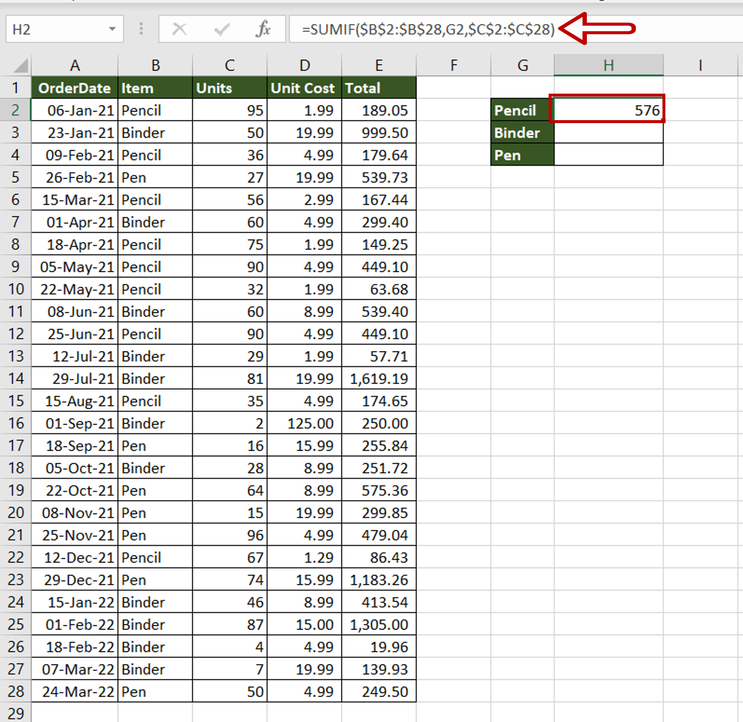
– In the destination cell, enter the formula using cell references:
= SUMIF($Item$,Pencil,$Units$)
– Make the ‘Item’ and ‘Units’ constant by selecting the cell references and pressing F4
– Press Enter
Step 2 – Copy the formula
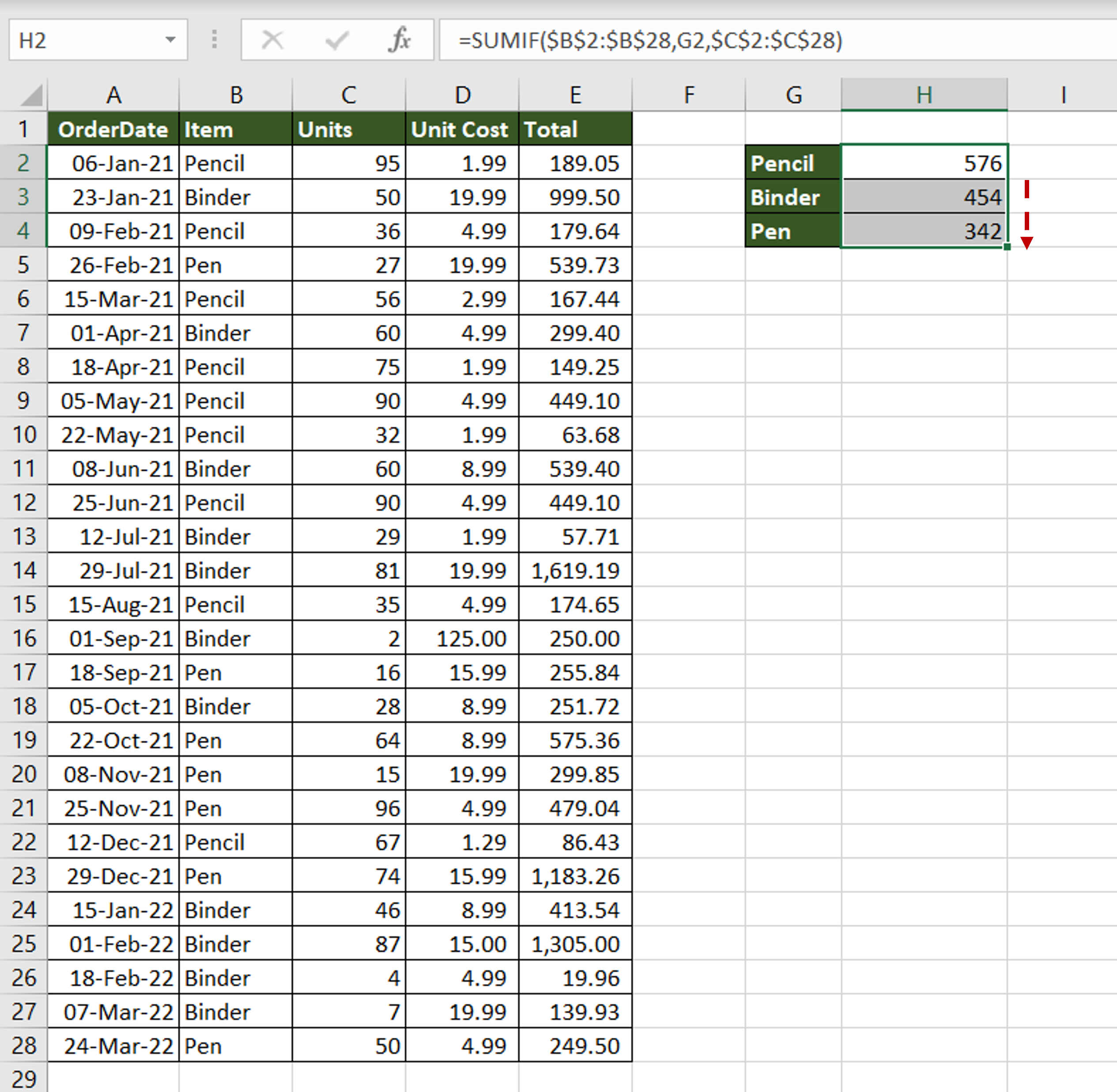
– Using the fill handle from the first cell, drag the formula to the remaining cells
OR
a) Select the cell with the formula and press Ctrl+C or choose Copy from the context menu (right-click)
b) Select the rest of the cells in the column and press Ctrl+V or choose Paste from the context menu (right-click)
Step 3 – Check the result
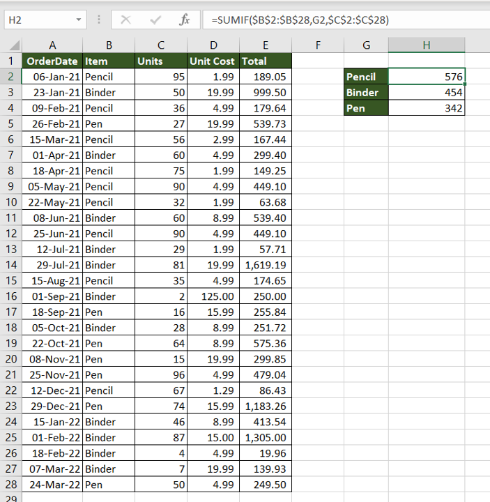
– A summary of the number of units required for each item is created


