
How to sum time in excel
 By
SpreadCheaters
By
SpreadCheaters
Microsoft Excel offers a very interesting way to sum time. The summing up is generic, all we need to do is change the format of the sum to get the actual summation result. We can perform the below mentioned way to perform sum time in excel:
We’ll learn about this methodology step by step.
Summing time in excel:
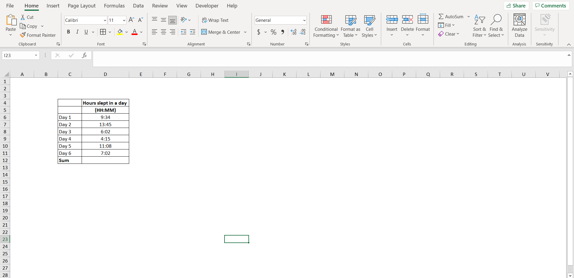
Step-1: Excel sheet with values containing time measurements
To do this yourself, please follow the steps described below;
– Open the desired Excel workbook with some data including entries of time which could be summed up
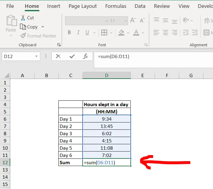
– Now calculate the sum of these time durations using a simple “=SUM()” formula, as shown in the image below.
Step-2: Calculating the sum of the time durations
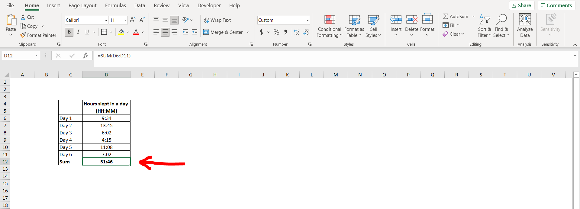
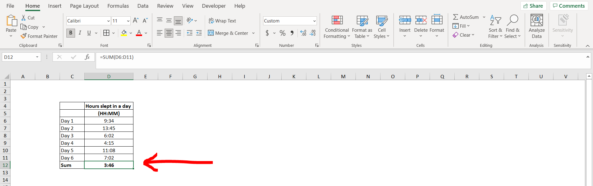
– Now we see that we have got the sum, but still it doesn’t look right. This is because by default, excel shows time in the 24 hour format, so no matter what the sum is, whenever the sum goes above 24 hour- mark, it comes back to 0.
Step-3: Getting the sum in 24-hour format
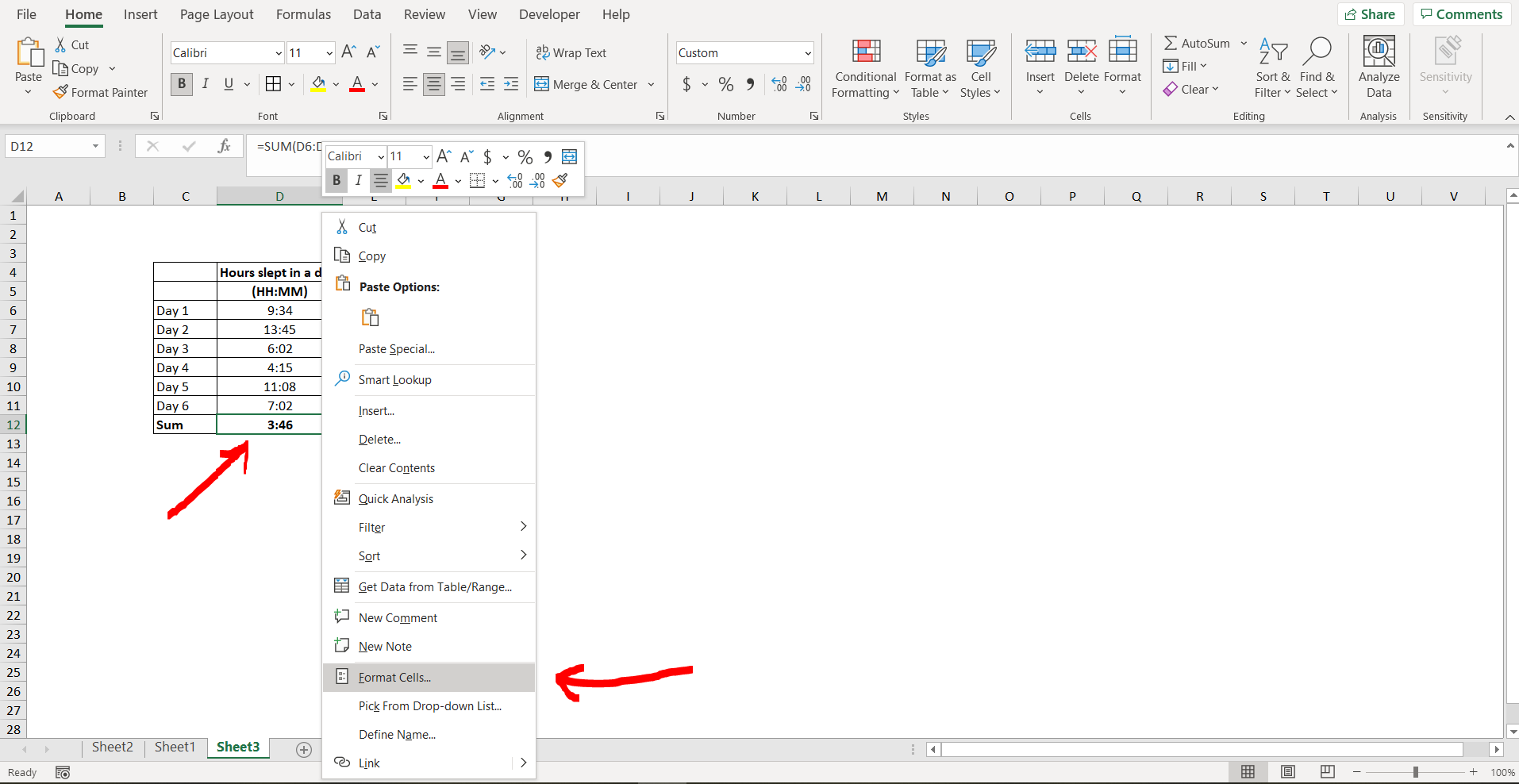
– To correct this, let’s go to the cell where the sum is calculated (in our case it is cell “D12”). Right click on this cell, and choose the “Format Cells” option, as displayed in the image below.
Step-4: Opening format cells option to change the format of the cell
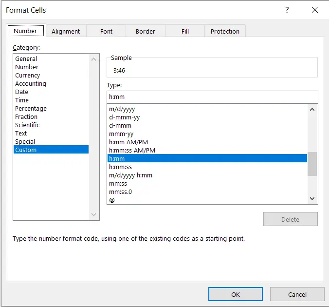
– A dialogue box appears. It shows what the current format of the cell is. We can see that currently, the format is in the custom category, and it is in “h:mm” format.
Step-5: Format cells dialogue box
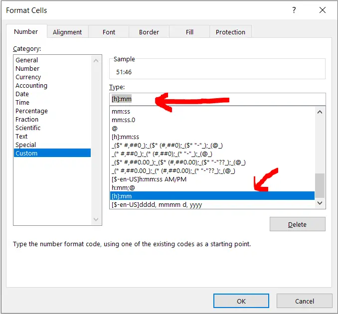
– We need to scroll through these options and select the “[h]:mm” option. Click “OK” once this option has been selected.
Step-6: Selecting the correct cell format
– Now we can see the correct summation of the time durations as depicted in the image below.
Final Image: Correct time format to show the sum
– Correct time format to show the sum


