
How to sum colored cells in Excel
 By
SpreadCheaters
By
SpreadCheaters
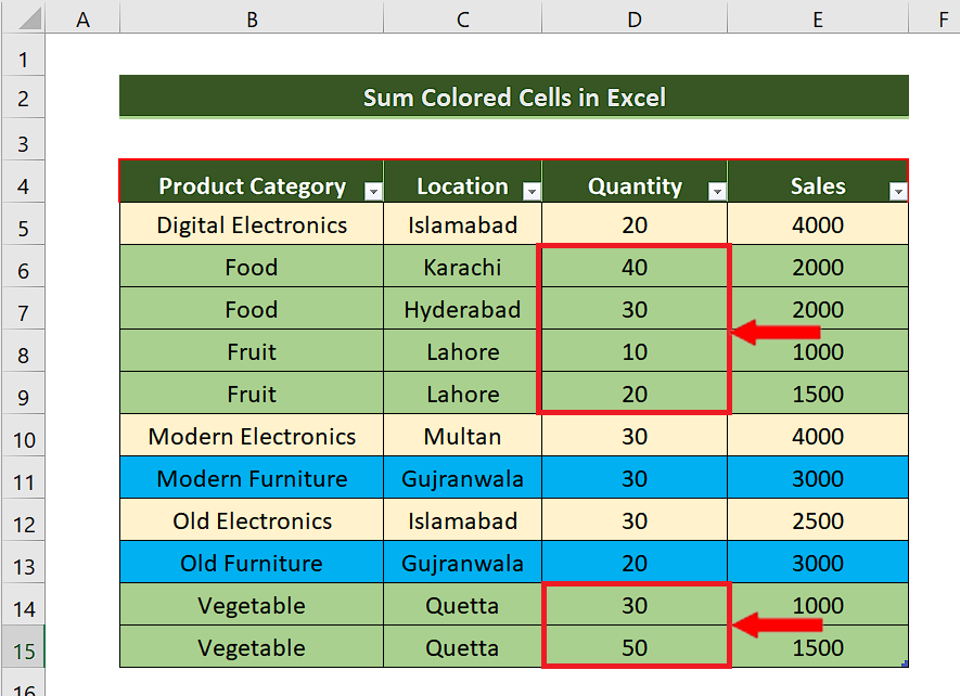
We are going to learn how to Sum Colored cells by all below mentioned methods in Excel. Let’s take a look at the following sales dataset shown above.
Sometimes to present the data in an aesthetic manner we have to use colorful themes to differentiate one type of data from others. There arises a requirement to sum the cells that have similar colors in some datasets like shown above. Microsoft Excel doesn’t provide us with a straightforward method to achieve this goal. However, we can get it done by using the following methods;
– Filter and SUBTOTAL
Step 1 – Apply the filter using shortcut key CTRL+SHIFT+L
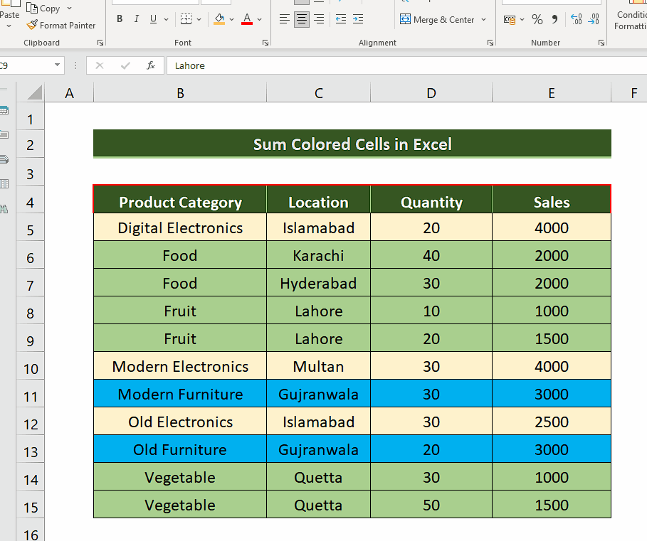
– Select a cell inside your dataset.
– Use the shortcut key to apply a filter to the dataset by pressing CTRL+SHIFT+L.
– This will apply the filter to all columns in the data range automatically.
– The same thing can also be done by going to the Sort & Filter option in the Editing group on the Home tab from the list of main tabs in Excel.
Step 2 – Use Filter by Color to filter rows in Excel

– We’ll go to the column header of interest, which in our case is the Product Category and click on the dropdown arrow.
– This will open up new options and we’ll click the Filter by Color option this will give us the option to choose between all the cell colors available in our data range. Since we want to choose the eatables which are in green color i.e., therefore, we’ll choose green color.
– Our data will be filtered and we’ll see only the green colored cells as shown above.
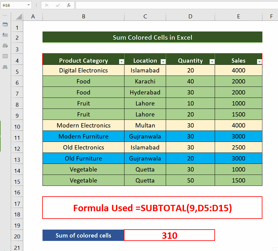
Step 3 – Use SUBTOTAL function to sum the colored cells only

– Now we’ll use the subtotal function to sum the colored cells as a result of application of the color filter. We’ll use the following simple formula;
=SUBTOTAL(9,D5:D15)
– In the above formula, we are adding the colored cells by adding the rows that contain numeric data of quantity.
This is how we can sum the colored rows in Excel by using Filter and SUBTOTAL together.


