
How to subtract rows in Excel.
 By
SpreadCheaters
By
SpreadCheaters
Performing row subtractions in Excel is a powerful feature that allows you to calculate the difference between values in different rows. Whether you need to analyze trends, track changes, or calculate variances, subtracting rows can provide valuable insights into your data.
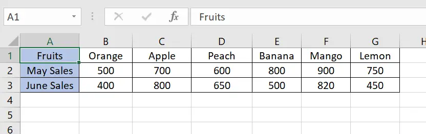
Suppose you have an Excel sheet containing Fruits and their Sales over the course of two months. The dataset includes the following rows: Fruits, May Sales, and June Sales. In this tutorial, we will explore different methods to subtract rows in Excel, empowering you to efficiently perform calculations and enhance your data analysis capabilities. Now let’s take a look at the Dataset.
Method – 1 Using Subtract formula.
This formula is useful when you need to calculate the difference between two-time values or numeric values. It allows you to perform calculations, adjustments, or comparisons that provide valuable insights into your data and facilitate various analysis tasks.
Step – 1 Select the cell.
- Select the row where you want to write the formula.
- This row will show the difference.
- The syntax of the formula will be
=First_Cell_Address-Second_Cell_Address
- In our case the formula will be
=B2-B3
Step – 2 Apply the formula.
- Press Enter to apply the formula.
- Use the Fill Handle to drag the formula down to apply it to other rows.
Method – 2 Using Array Formula.
This formula is an array of values, representing the differences between the corresponding cells in the first and second ranges. Each cell in the resulting array contains the subtraction result for the corresponding pair of cells in the ranges.
Step – 1 Select the cells and write the formula
- Select all the cells in the row where you want to write the formula, if you are using Excel 2019 or below. If you are using Excel 365 or Excel 2021 then you can select the first cell only.
- The syntax of the formula will be
=(First_Cell_Address:Second_Cell_Address-Third_Cell_Address:Fourth_Cell_Address)
- In our case, the formula will be
=(B2:G2-B3:G3)
Step – 2 Apply the formula
- Press Ctrl + Shift + Enter to apply the formula. The array formula will calculate the results for all the entries in the rows.


