How to standardize data in Excel
You can watch a video tutorial here.
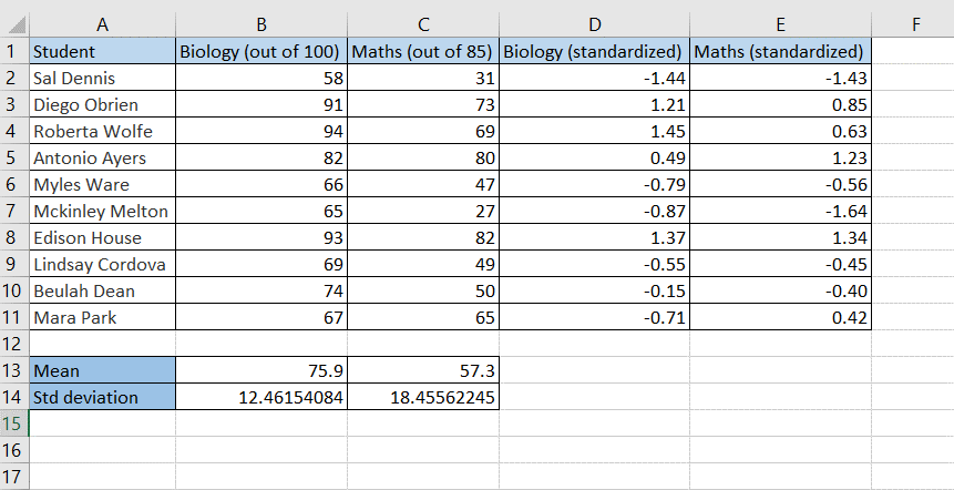
Standardizing data is the process of rescaling the values in a dataset to a common scale so that it can be compared to other datasets or to understand the variance in the values. This is commonly used in machine learning to compare datasets that have different scales or units of measurement. In Excel, this can be done using the following functions:
1. AVERAGE(): this returns the mean of a set of values
a. Syntax: AVERAGE(range)
i. range: the range of values
2. STDEV.P(): this returns the standard deviation of a set of numbers
a. Syntax: STDEV.P(range)
i. range: the range of values
3. STANDARDIZE(): this returns a standardized value based on the mean and standard deviation of the dataset
a. Syntax: STANDARDIZE(number, mean, std)
i. number: the number to be standardized
ii. mean: the mean of the dataset
iii. std: the standard deviation of the dataset
Step 1 – Calculate the mean of each set of data
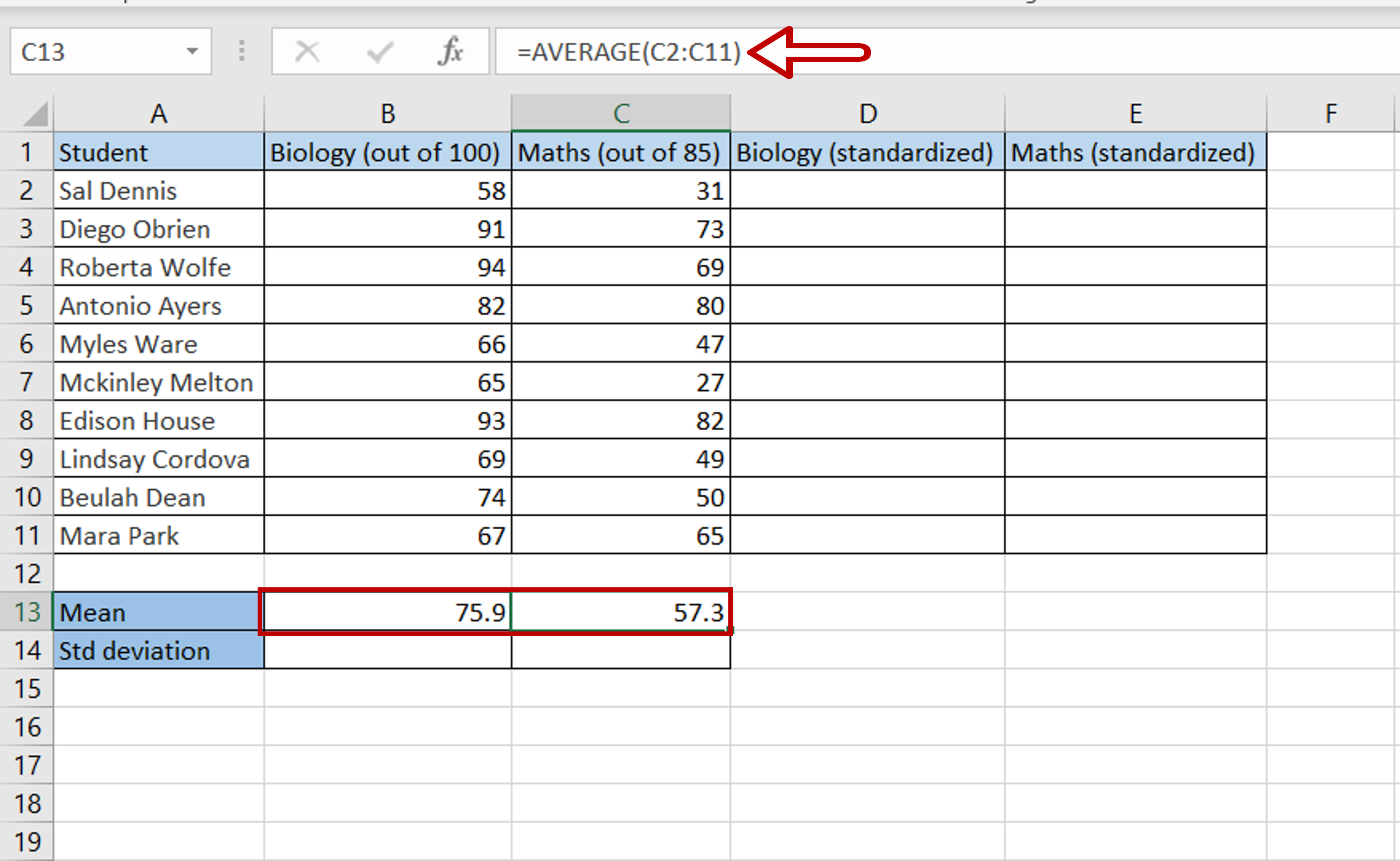
– Select the destination cell
– Type the formula using cell references:
=AVERAGE(range of Biology (out of 100))
– Press Enter
– Select the destination cell
– Type the formula using cell references:
=AVERAGE(range of Maths (out of 85))
– Press Enter
Step 2 – Calculate the standard deviation of each set of data
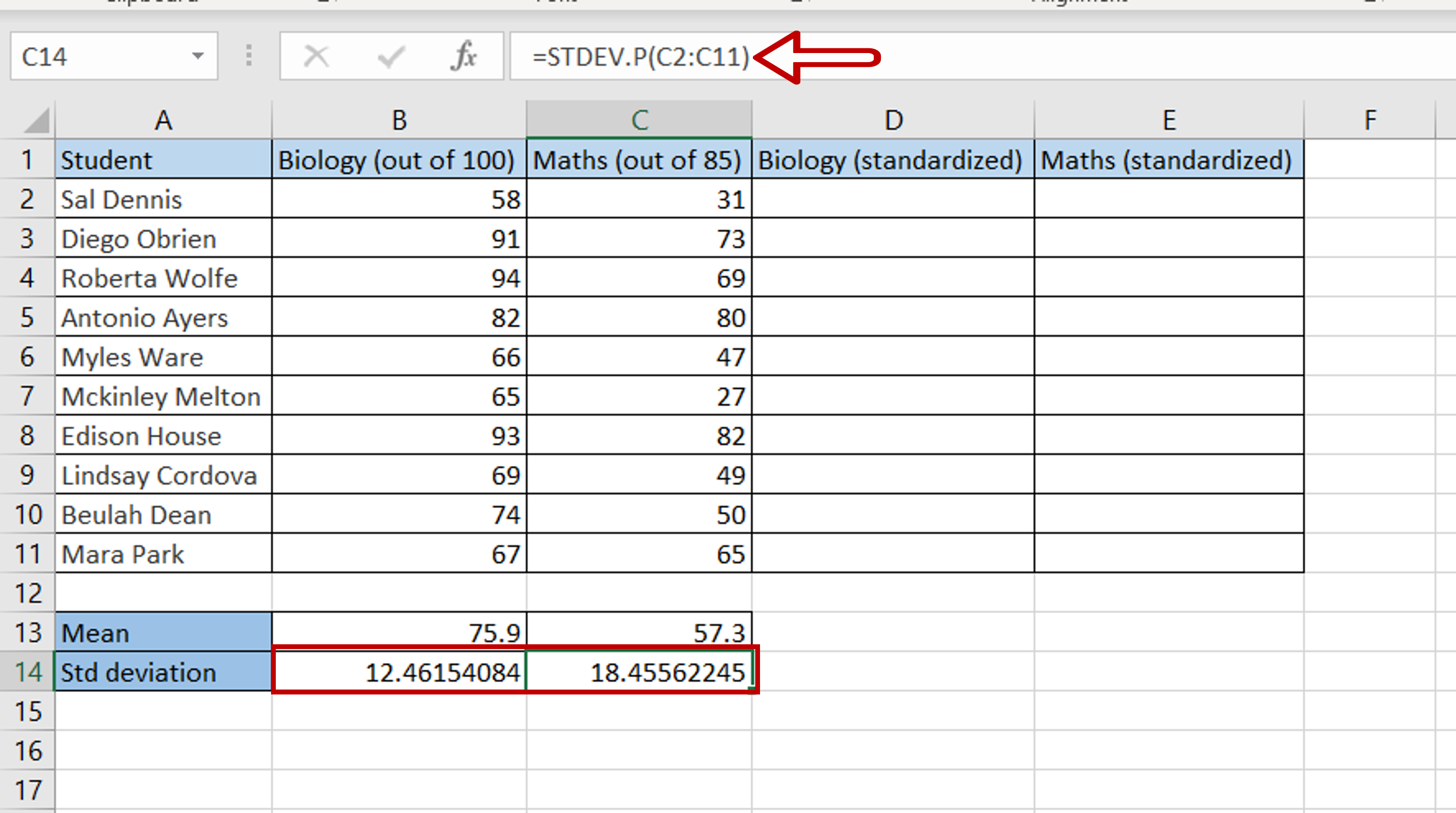
– Select the destination cell
– Type the formula using cell references:
=STDEV.P(range of Biology (out of 100))
– Press Enter
– Select the destination cell
– Type the formula using cell references:
=STDEV.P (range of Maths (out of 85))
– Press Enter
Step 3 – Create the formulas for standardization
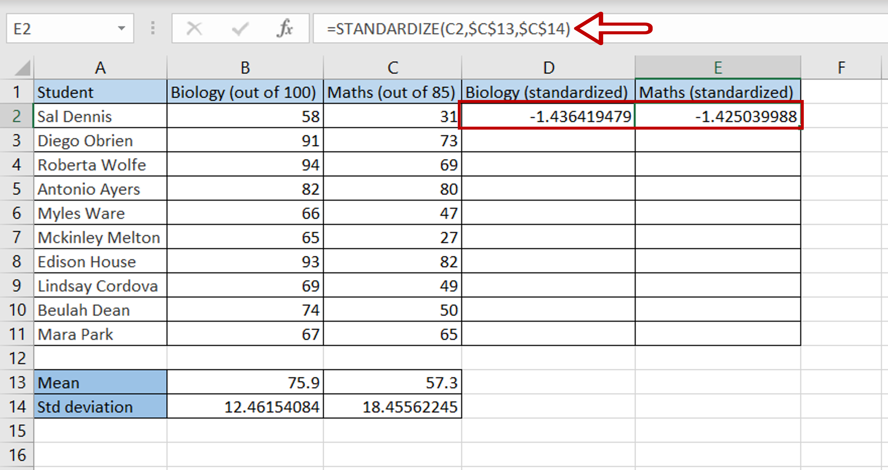
– Select the destination cell
– Type the formula using cell references:
=STANDARDIZE(Biology (out of 100), $Mean$, $Std deviation$)
– Press Enter
– Select the destination cell
– Type the formula using cell references:
=STANDARDIZE( Maths (out of 85), $Mean$, $Std deviation$)
– Press Enter
– In both formulas, make the ‘Mean’ and ‘Std deviation” constant by selecting the cell references and pressing F4 to add the dollar signs ($)
Step 4 – Copy the formulas
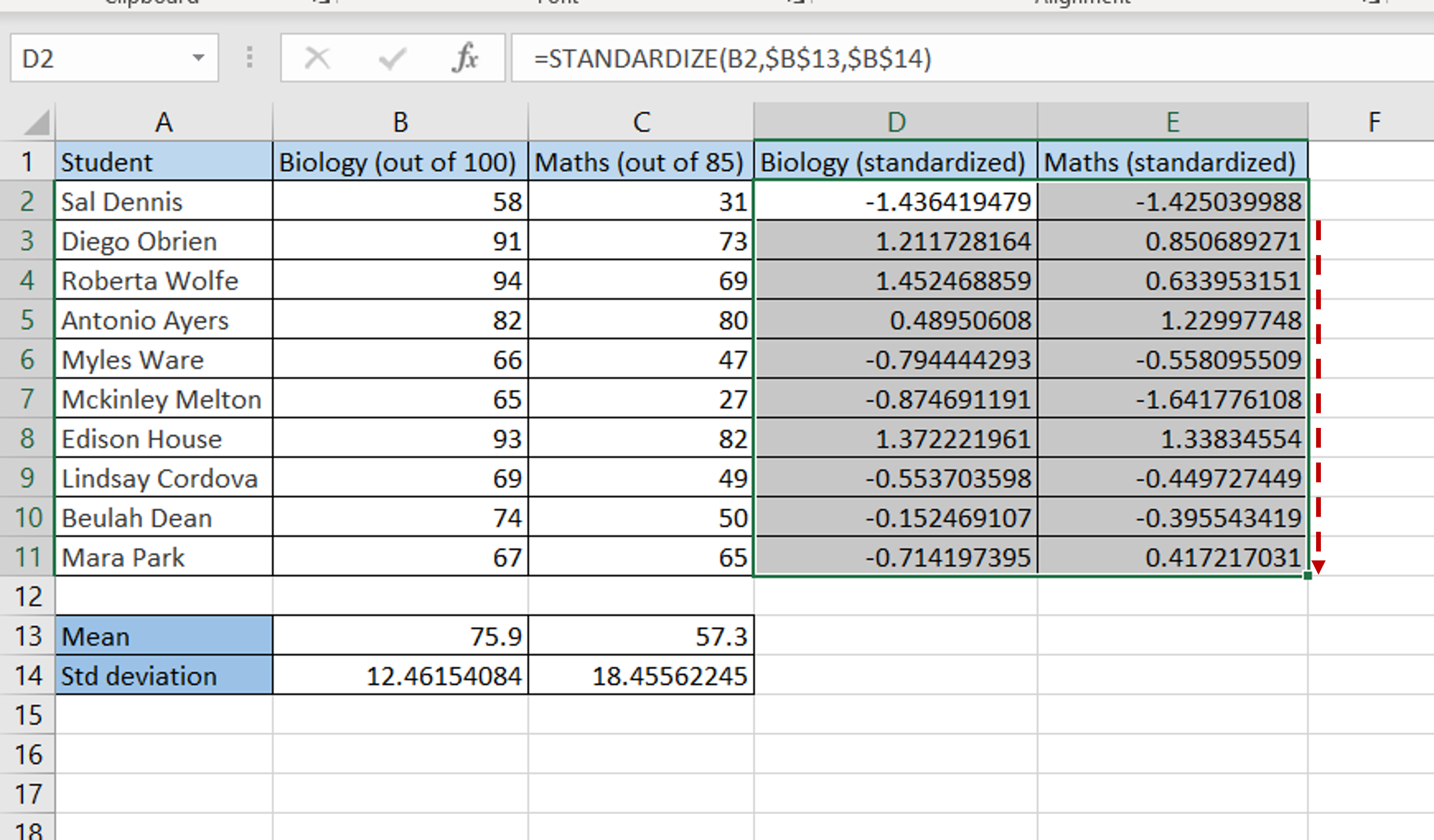
– Select the cells with the formulas
– Using the fill handle, drag the formula to the remaining cells
OR
a. Select the cell with the formula and press Ctrl+C or choose Copy from the context menu (right-click)
b. Select the rest of the cells in the column and press Ctrl+V or choose Paste from the context menu (right-click)
Step 5 – Check the result
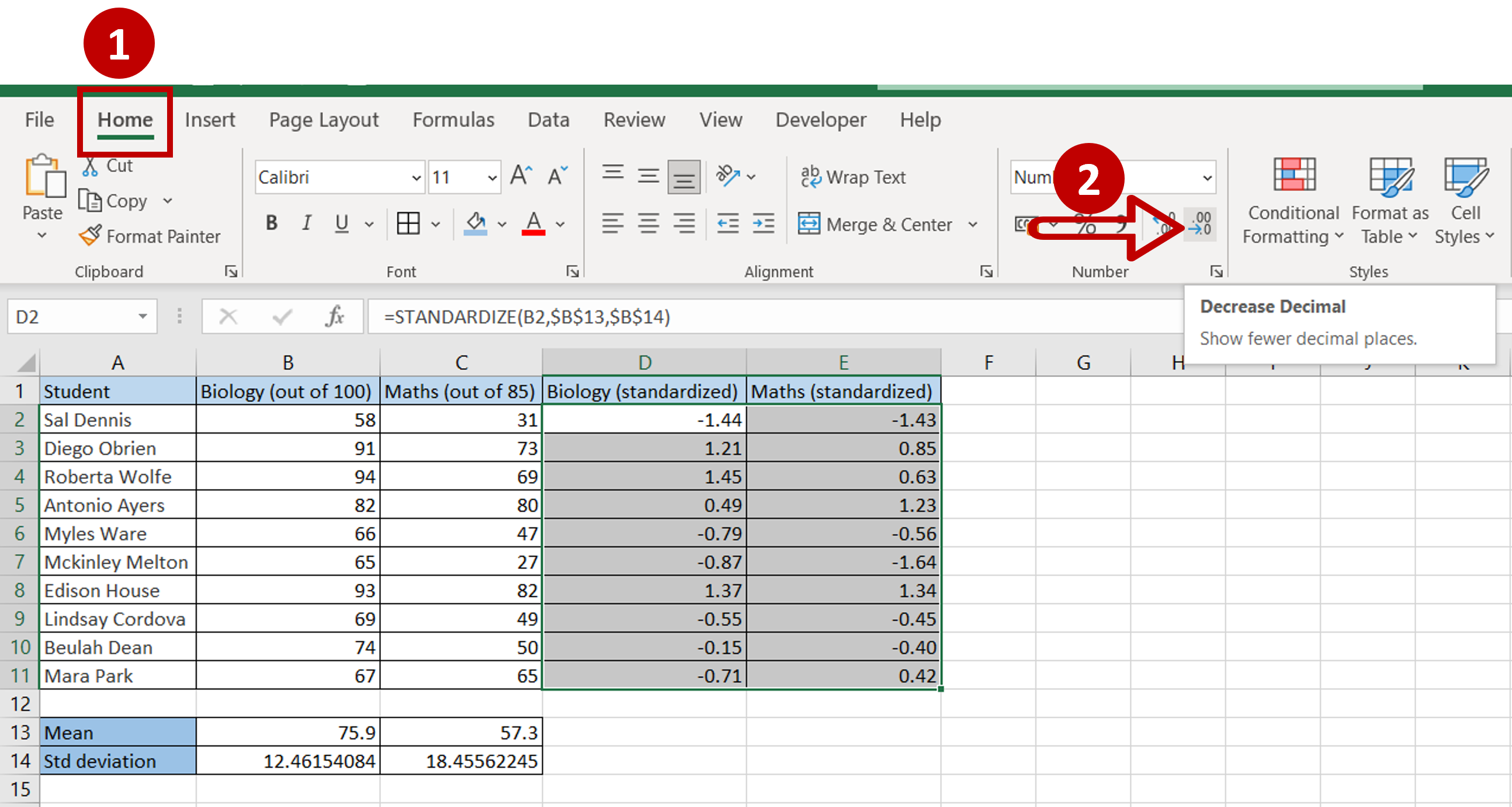
– Go to Home > Number
– Click on the Decrease Decimal button
– Each dataset has been scaled to standardized values
– Each student’s performance in each subject can now be compared


