
How to square a number in Excel
 By
SpreadCheaters
By
SpreadCheaters
Page last updated:
23/06/2023 |
Next review date:
23/06/2025
You can watch a video tutorial here.
Excel is a very powerful tool when it comes to performing mathematical calculations on numeric data. It provides versatile functions to conduct calculations ranging from basic to complex.
In this tutorial we’ll learn how to calculate the square of a number in Excel. This can be done by two methods.
- By simple multiplication
- By using caret symbol
- By using Power Formula
Let’s explore all these methods one by one.
Method 1 By Simple Multiplication
Step 1 – Multiply the number by itself
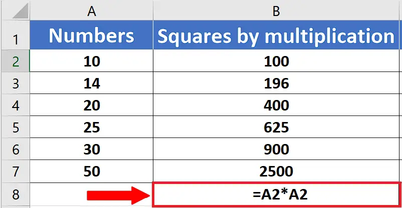
- The simplest of all methods to take a square of the number is to multiply the number by itself. So let’s use simple multiplication by using * multiplication symbol and writing the following formula in an appropriate cell.
=A2*A2
- This will give us the square of the number in A2 cell. Double click the fill handle to fill the rest of the rows with the same formula.
Method 2 By Using Caret ^ Symbol
Step 1 – Use Caret symbol ^ to take 2nd Power (square) of number
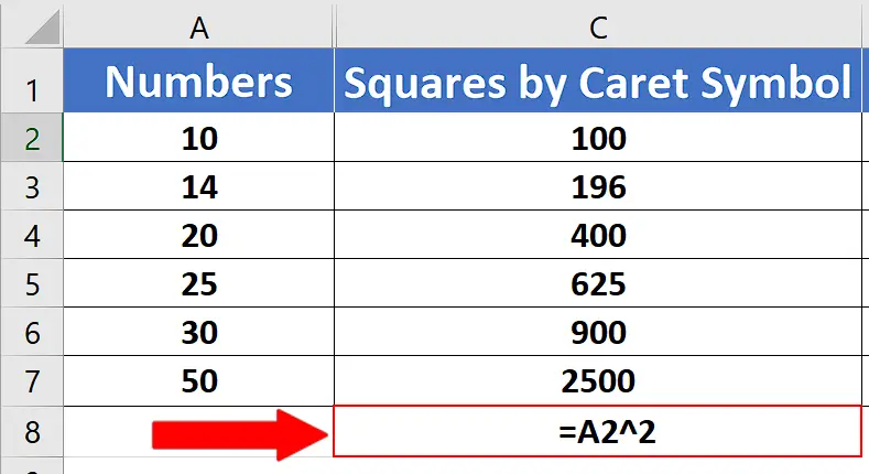
- The second method to take the square of the number is to use the Caret Symbol (^) to calculate the 2nd power of the number which is equal to the square of that number.
- For this purpose we’ll write =A2^2 in C2. This will give us the square of the number in A2 cell.
- Double click the fill handle to fill the rest of the rows with the same formula.
Method 3 By Using POWER Function
Step 1 – Use POWER function to take 2nd Power (square) of number
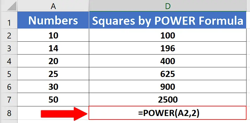
- The third and last method is to use the POWER function which is a built-in function of Excel. We’ll write the formula in cell D2.
=POWER(A2, 2)
- This will give us the square of the number in A2 cell. Double click the fill handle to fill the rest of the rows with the same formula.


