
How to split a cell into two rows in Excel
 By
SpreadCheaters
By
SpreadCheaters
You can watch a video tutorial here.

Working with data in Excel frequently involves manipulating and organizing data. You may find a situation where you need to split a cell into two rows. This can be done by using the Text to Columns tool in combination with the transpose operation in Excel.
Step 1 – Analyze the data
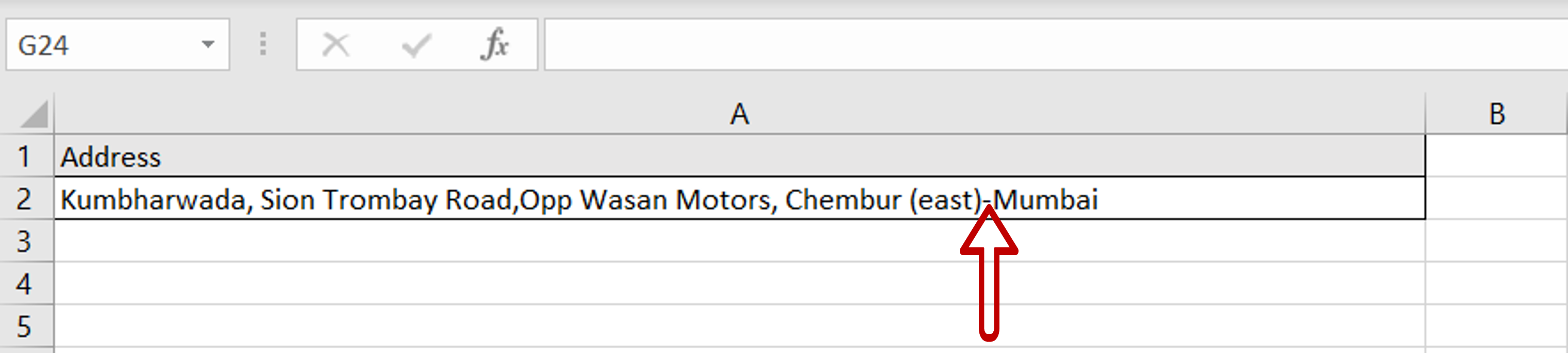
– Check the cell to see how the text is to be separated
– In this example, the text is separated by a hyphen (-)
Step 2 – Open the Convert Text to Columns Wizard
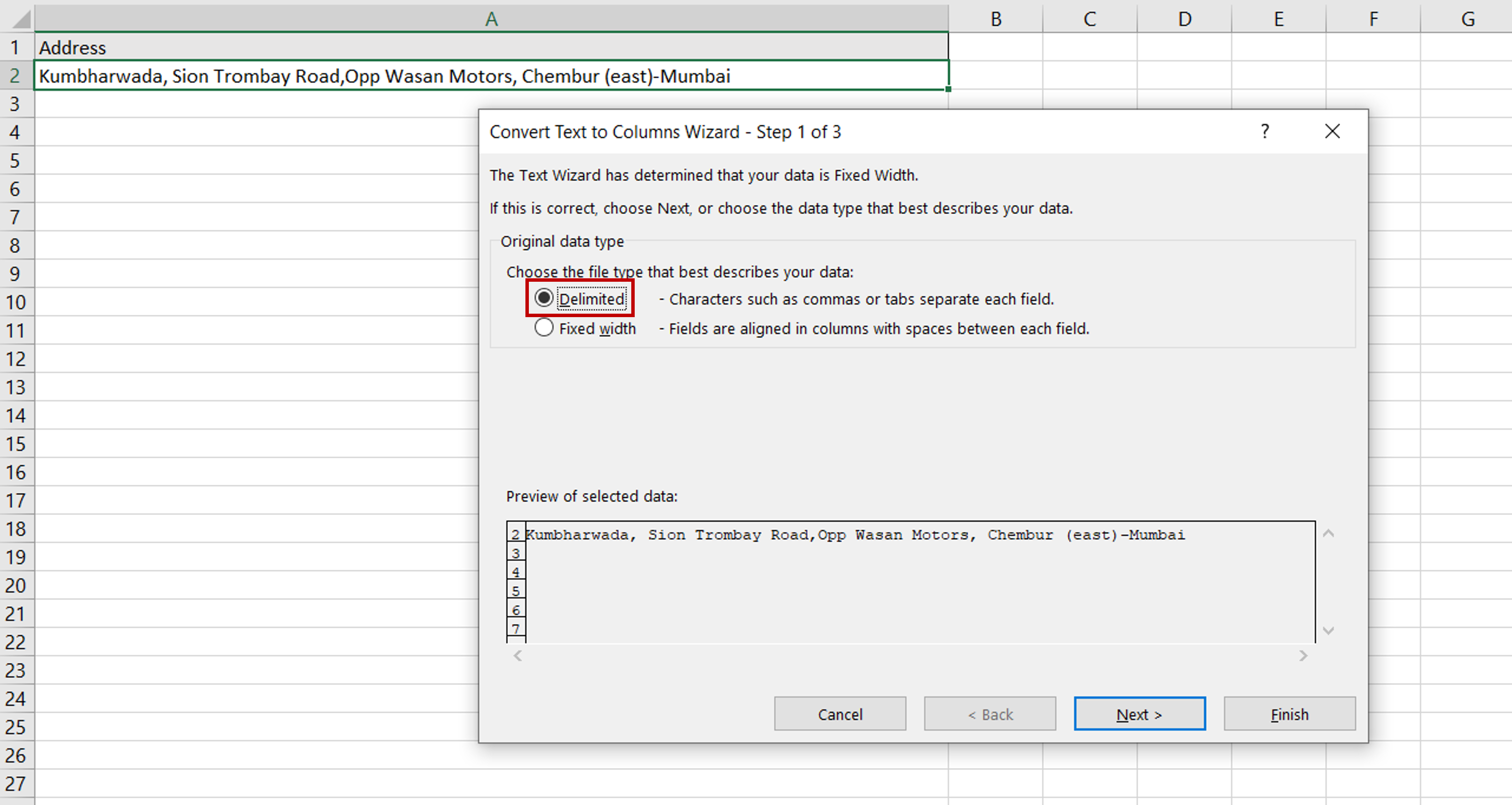
– Select the cell
– Go to Data > Data Tools
– Click on Text to Columns
– Select the Delimited option as the addresses are separated (or delimited) by a hyphen
– Click on Next
Step 3 – Choose the delimiter
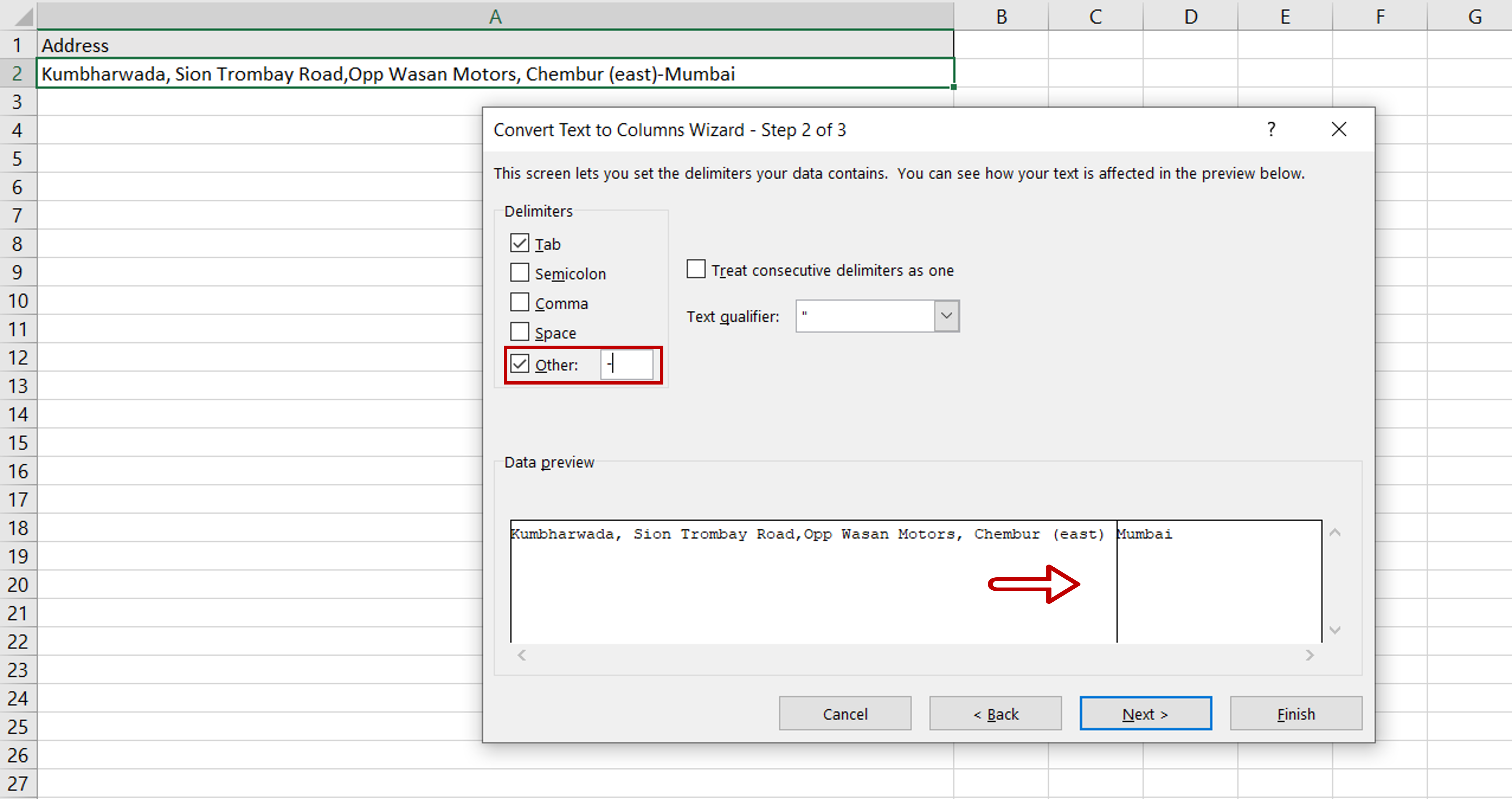
– Under Delimiters, choose Other and type in a hyphen(-)
– Check how the data has been separated in the Data preview
Step 4 – Choose the format and destination
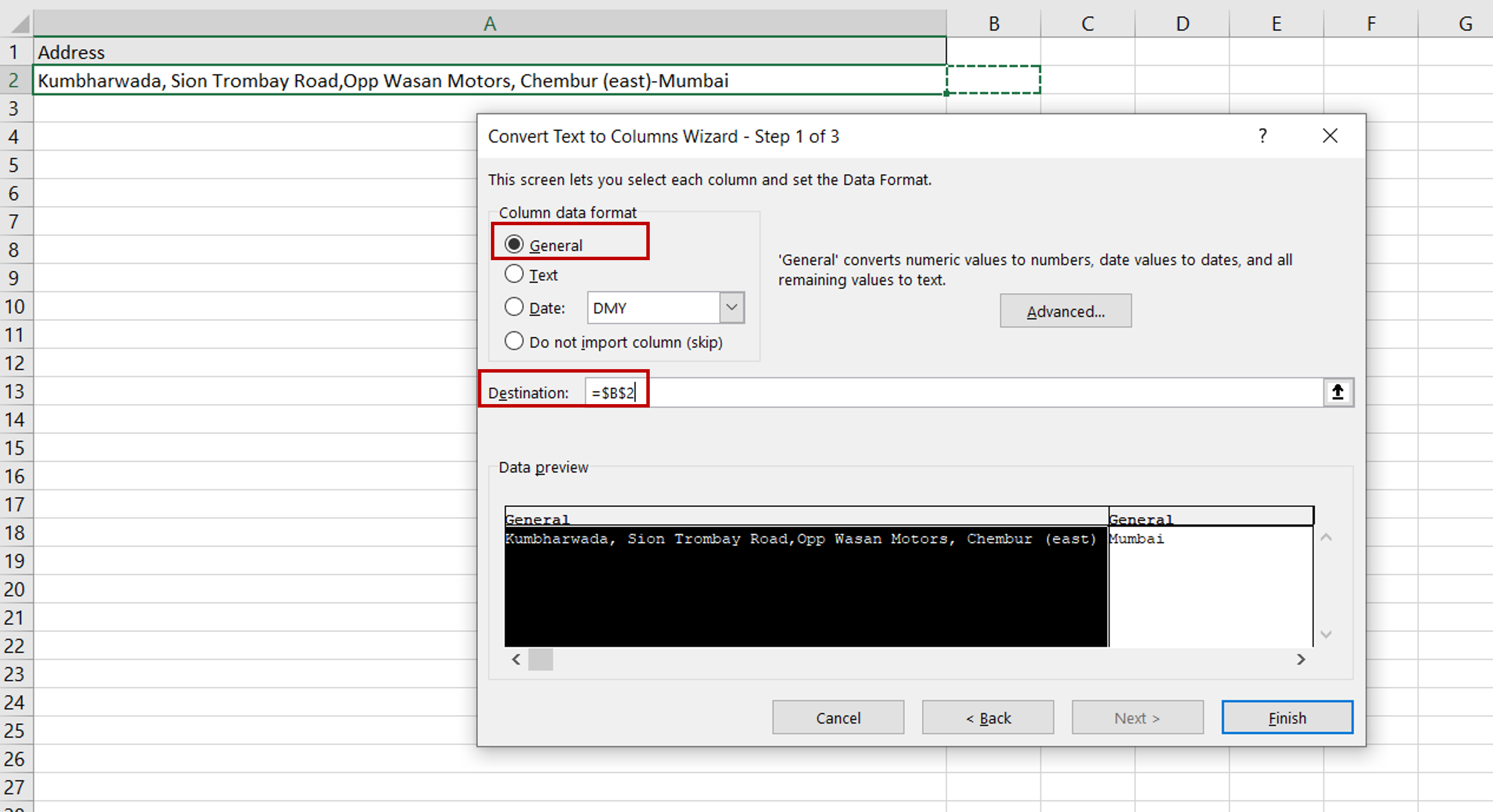
– Under Column data format, choose General
– Select the Destination for the data
– Click Finish
Step 5 – Open the Paste Special window
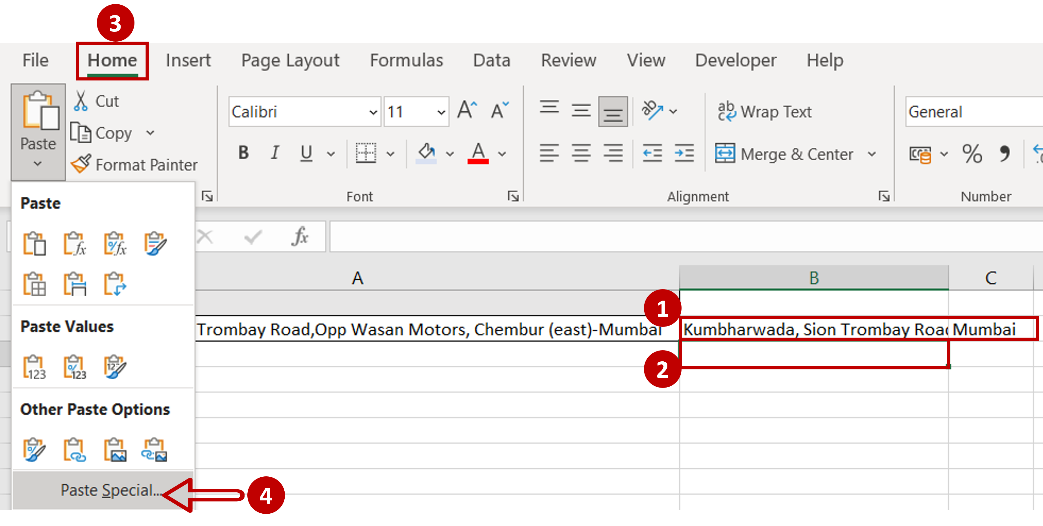
– Copy the split data
– Select the destination for the rows
– Go to Home > Paste > Paste Special
Step 6 – Transpose the data
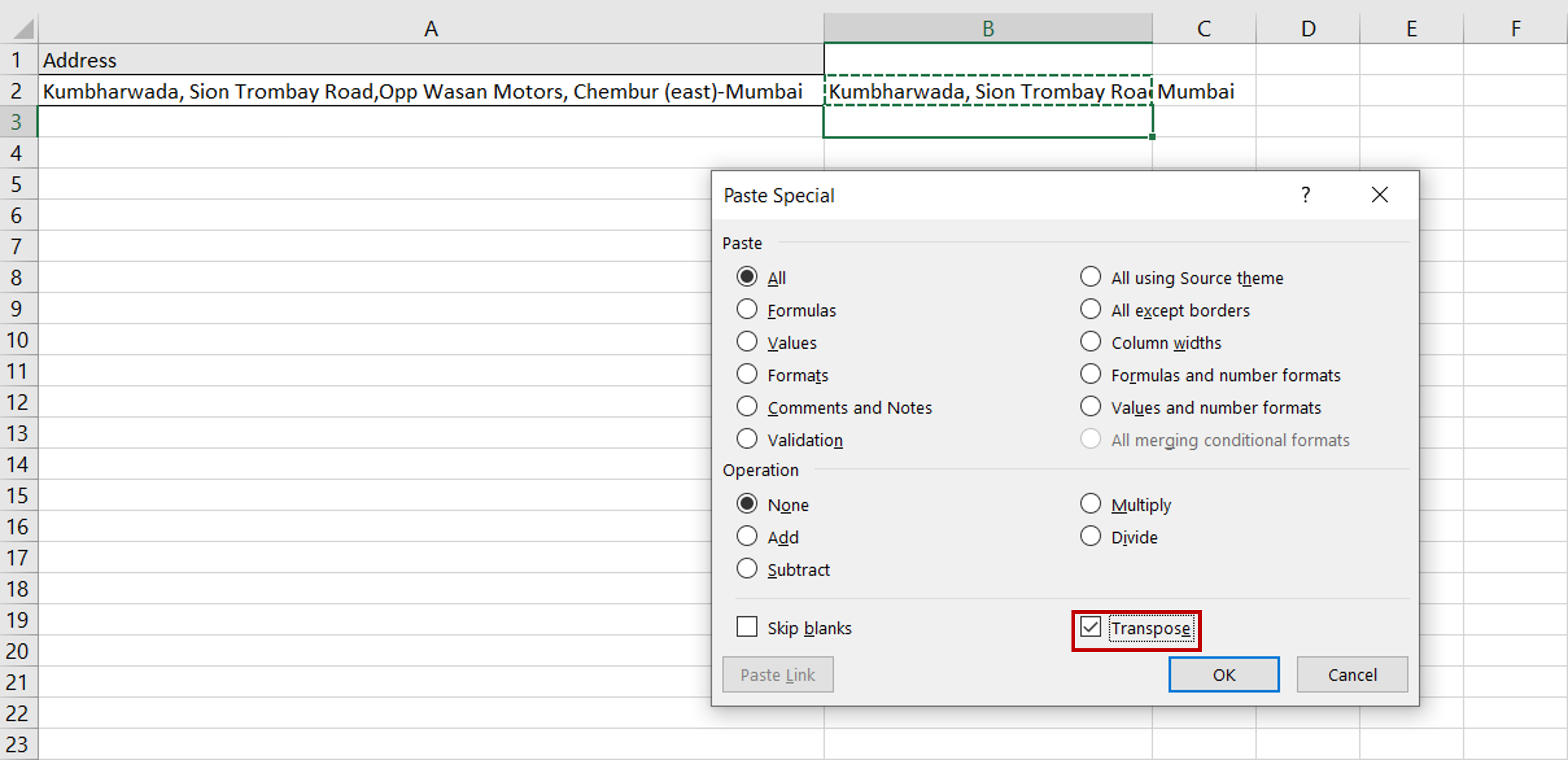
– Select transpose
– Click OK
Step 7 – View the result
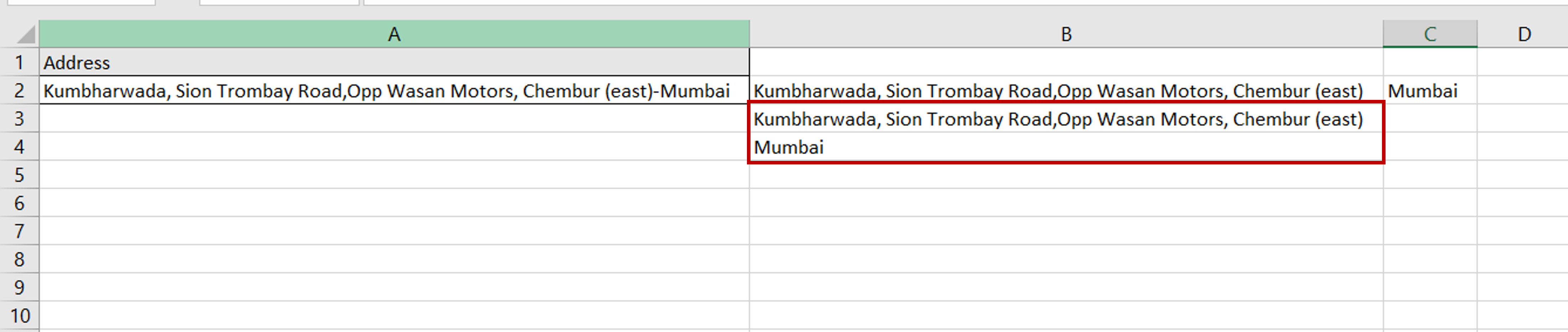
– The data from one cell has been split into two rows


