
How to sort Grand Total in PivotTable
 By
SpreadCheaters
By
SpreadCheaters
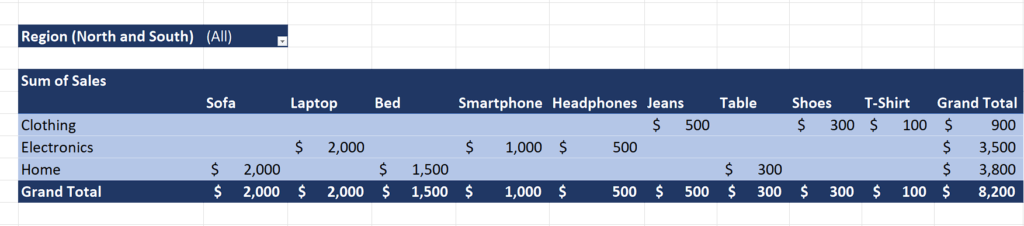
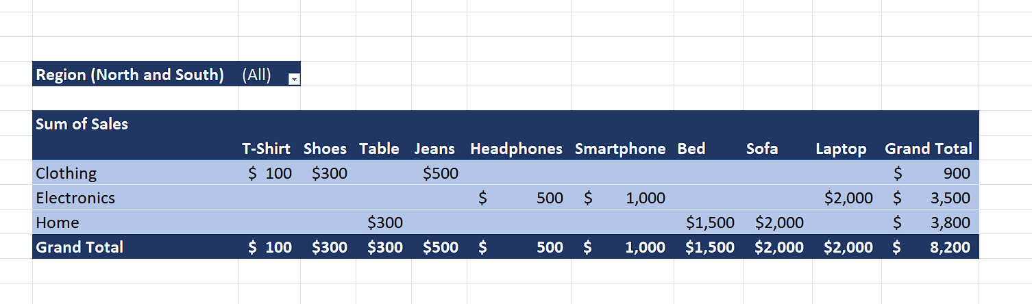
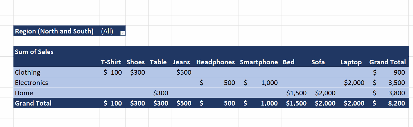
This sales report showcases diverse product sales across regions. Electronics, including smartphones and laptops, achieved sales of $1,000 and $2,000 respectively. Clothing items like T-shirts, jeans, and shoes generated sales of $100, $500, and $300. Home products, such as beds and sofas, achieved sales of $1,500 and $2,000. The Grand Total of the sales is $8,200. The report highlights regional variations in product performance. We will take this PivotTable as an example and learn how to sort the Grand Total.
Sorting the Pivot table by the grand total allows you to quickly identify the highest or lowest values across different categories or dimensions. This can be helpful when you want to find the top-selling products, the most productive employees, or the regions with the highest revenue.
Step 1 – Select the cell
– Select any cell that contains the Grand Total value for a specific product.
Step 2 – Sort the PivotTable by Grand Total
– Now, Right-click on the selected cell and it will open a context menu.
– Hover your mouse over the “Sort” option.
– Now, sort the “Grand Total” by “Largest to Smallest” or “Smallest to Largest” value.
– We are selecting the “Largest to Smallest” value because we wish to see the most sold product first.


