How to show tracer arrows in Excel

Tracer arrows, also known as formula arrows, are visual indicators in Microsoft Excel that display the relationships between cells used in a formula. There are two types of tracer arrows: Trace Precedents Arrows and Trace Dependents Arrows. These arrows are essential for understanding the connections between cells within a worksheet.

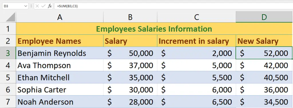
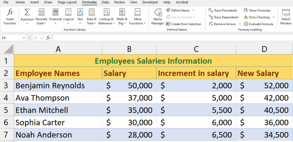
The dataset provided contains information about the salaries of five employees. Each row in the dataset represents an individual employee and includes their name, current salary, the increment in their salary, and the new salary after the increment which is calculated by summing the current salary and increment in their salary by SUM Function. We want to show tracer arrows to understand the connections between these cells.

There are two simple methods to do this which are as follows:

Method 1 – By using the Trace Precedents Option

The “Trace Precedents” arrows assist in illustrating the relationship between cells when a formula in one cell depends on the values or formulas in other cells.

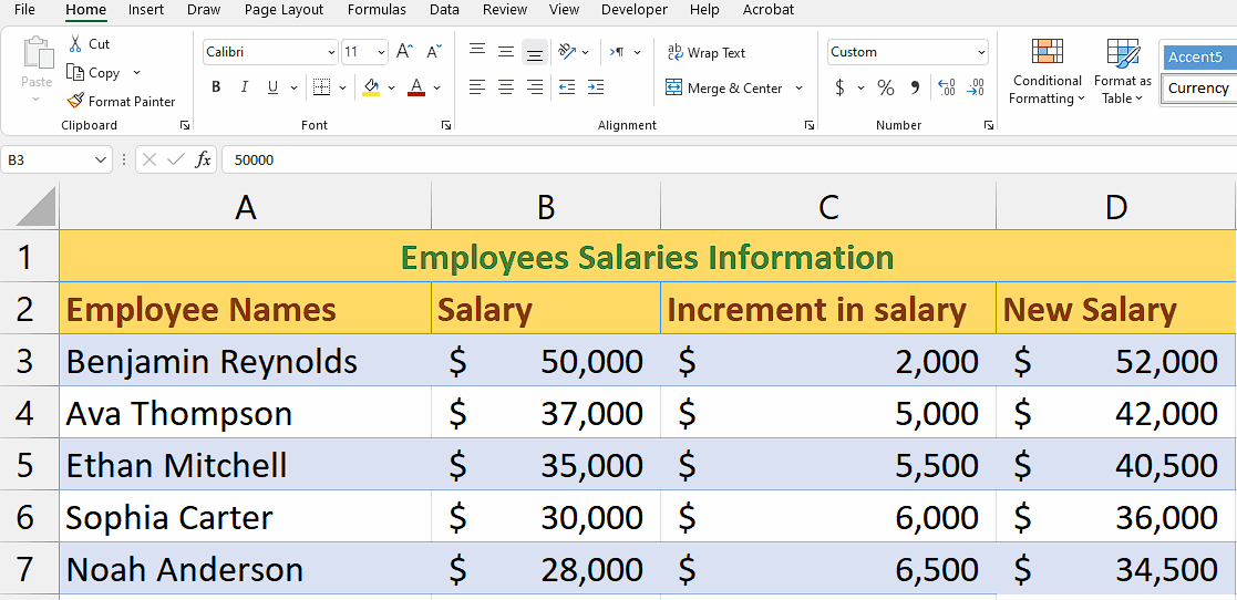
Step 1 – Select the cell

• Select the cell that contains the formula and uses the values of other cells to give the result.
• For instance, cell D3 contains the formula that sums the values of B3 and C3.

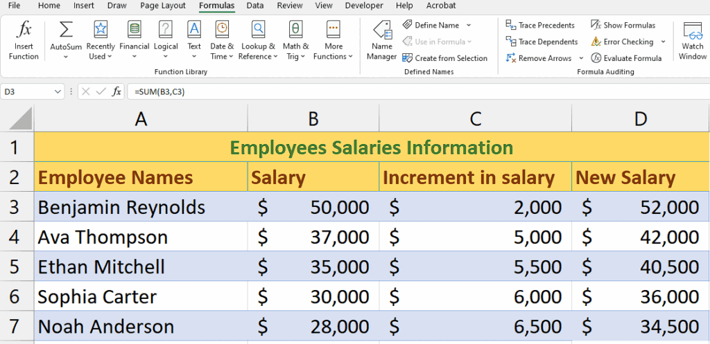
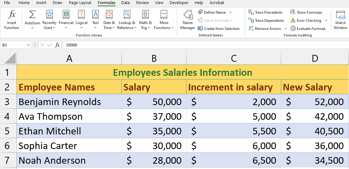
Step 2 – Navigate to Formulas Tab

• Open Microsoft Excel on your computer.
• Look for the ribbon at the top of the Excel window. The ribbon contains various tabs.
• Locate the “Formulas” tab on the ribbon
• Click on the “Formulas” tab. This action will switch the Excel interface to display the options and features available within the Formulas tab.

Step 3 – Show Tracer Arrows

• Look for the option named “Trace Precedents Option” under the “Formula Auditing” Group.
• Click on this option and tracer arrows will automatically appear.

Method 2 – By using Trace Dependents Option

This option draws trace arrows in the form of blue arrows to trace the cells that depend on their value to perform further operations.

Step 1 – Select the cell

• Select the cell that contains the values that are being used by other cells to give the result.
• For instance, cell B3 contains the value that is summed with C3 to give the result in D3.

Step 2 – Navigate to Formulas Tab

• Open Microsoft Excel on your computer.
• Look for the ribbon at the top of the Excel window. The ribbon contains various tabs.
• Locate the “Formulas” tab on the ribbon
• Click on the “Formulas” tab. This action will switch the Excel interface to display the options and features available within the Formulas tab.

Step 3 – Show Tracer Arrows

• Look for the option named “Trace Dependents Option” under the “Formula Auditing” Group.
• Click on this option and tracer arrows will automatically appear.