How to shade every other row in Excel
In this tutorial we will learn how to shade every other row in Excel. To do it yourself we will start with an example. We have a data range and we will color every other row by using conditional formatting with a specific formula.
Following is the step to follow:

Excel is a very powerful tool for data computing. In most of the cases, we face difficulty in organizing the data, adding color to specific rows and columns for the differentiation purposes.
Coloring alternate arrows in Excel spreadsheet is one of the simplest way to make the sheet user friendly. It improves readability and reduces clutter in the spreadsheet.
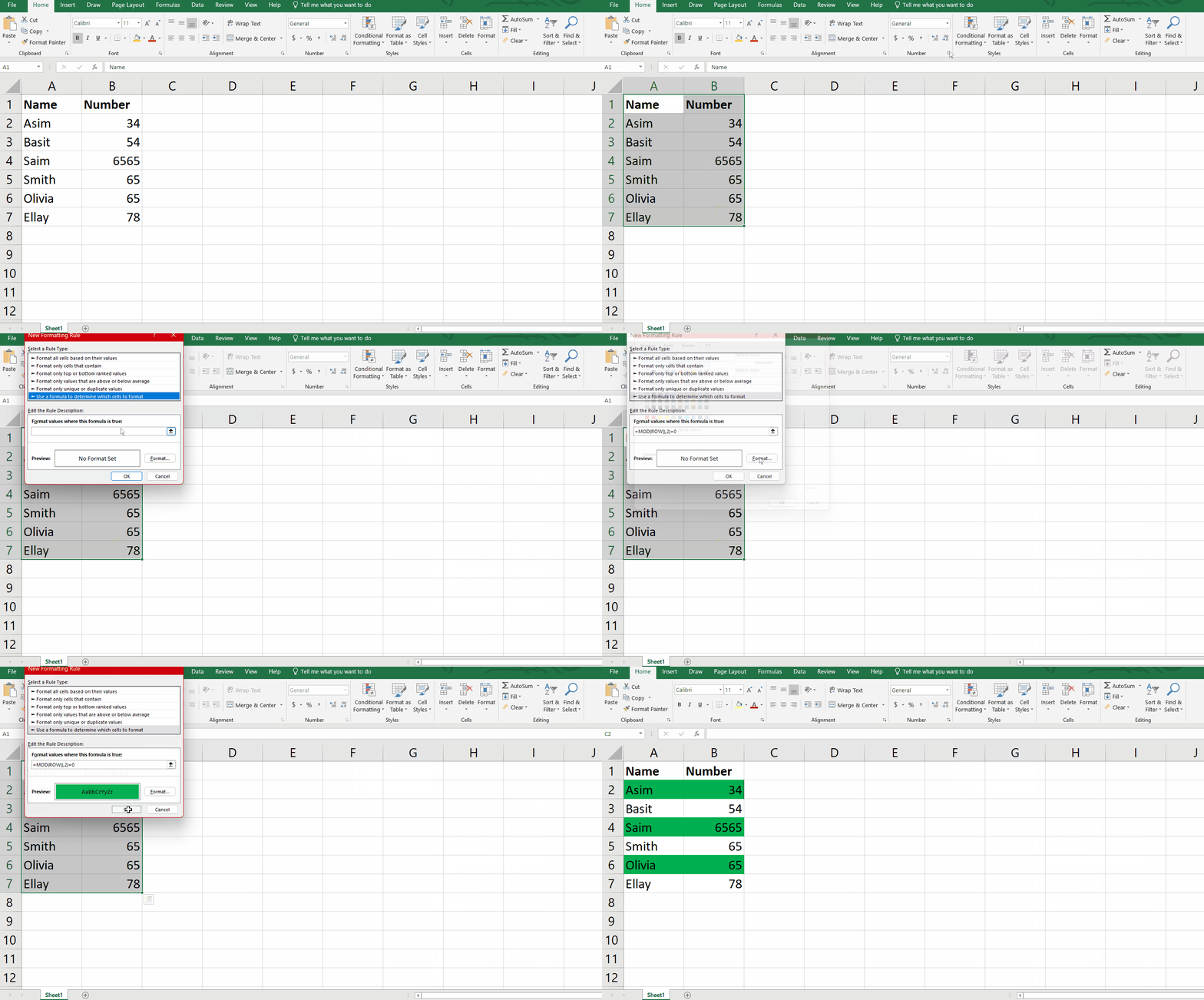
Step 1 – Select the data and apply formula

Above is an animation as an example.
– We have a specific range of data. Click on the Home tab then click Conditional formatting.
– Drop down menu will appear and click on New rule.
– Another dialogue box will open click on Use the formula to determine which cell to format.
– Write this formula in the text tab
=MOD(ROW() , 2)=0.
The row function returns the row number. The Mod function returns the remainder when the row is divided by 2. In the case of an even number it will return value 0 (FALSE). In case of every odd row it will return value 1 (TRUE). So all odd numbered rows will be highlighted with the desired color.
– Click on the Format button at the bottom right corner of the dialog box and select the fill tab.
– Select the color and Click OK.
– As soon as you press the enter key the alternative rows will be shaded with selected color.
Resultantly , we added color in alternate rows by using conditional formatting
Bonus tip : Use =MOD(COL(),2)=0 for column coloring.


