
How to separate information in Excel
 By
SpreadCheaters
By
SpreadCheaters
You can watch a video tutorial here.
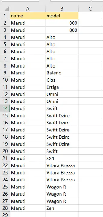
Excel has several tools and functions that can be used to manipulate data. These prove useful when you are cleaning data or consolidating data from multiple sources. When working with a dataset you may find that you need to separate the information in a single column into multiple columns. In this example, we are going to separate the manufacturer and model of the car from the column.
Step 1 – Open the Convert Text to Columns Wizard
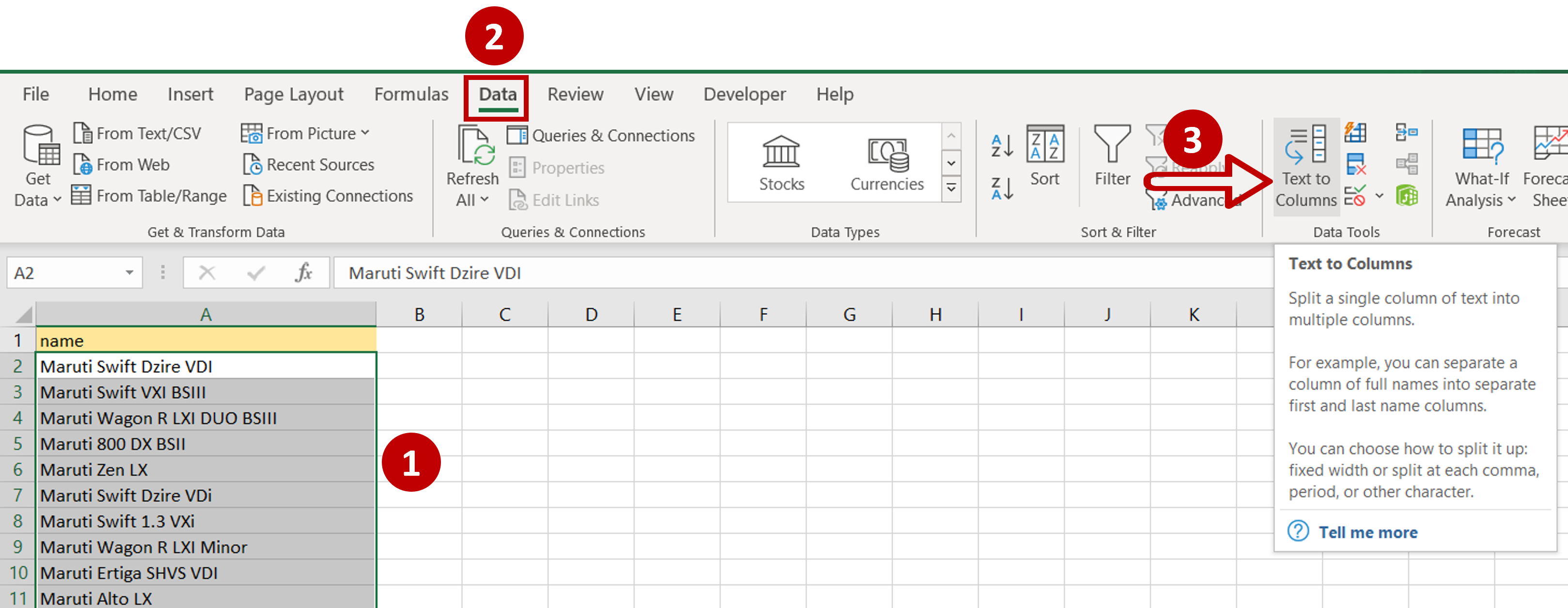
– Select the data
– Go to Data > Data Tools
– Click on Text to Columns
Step 2 – Choose the file type
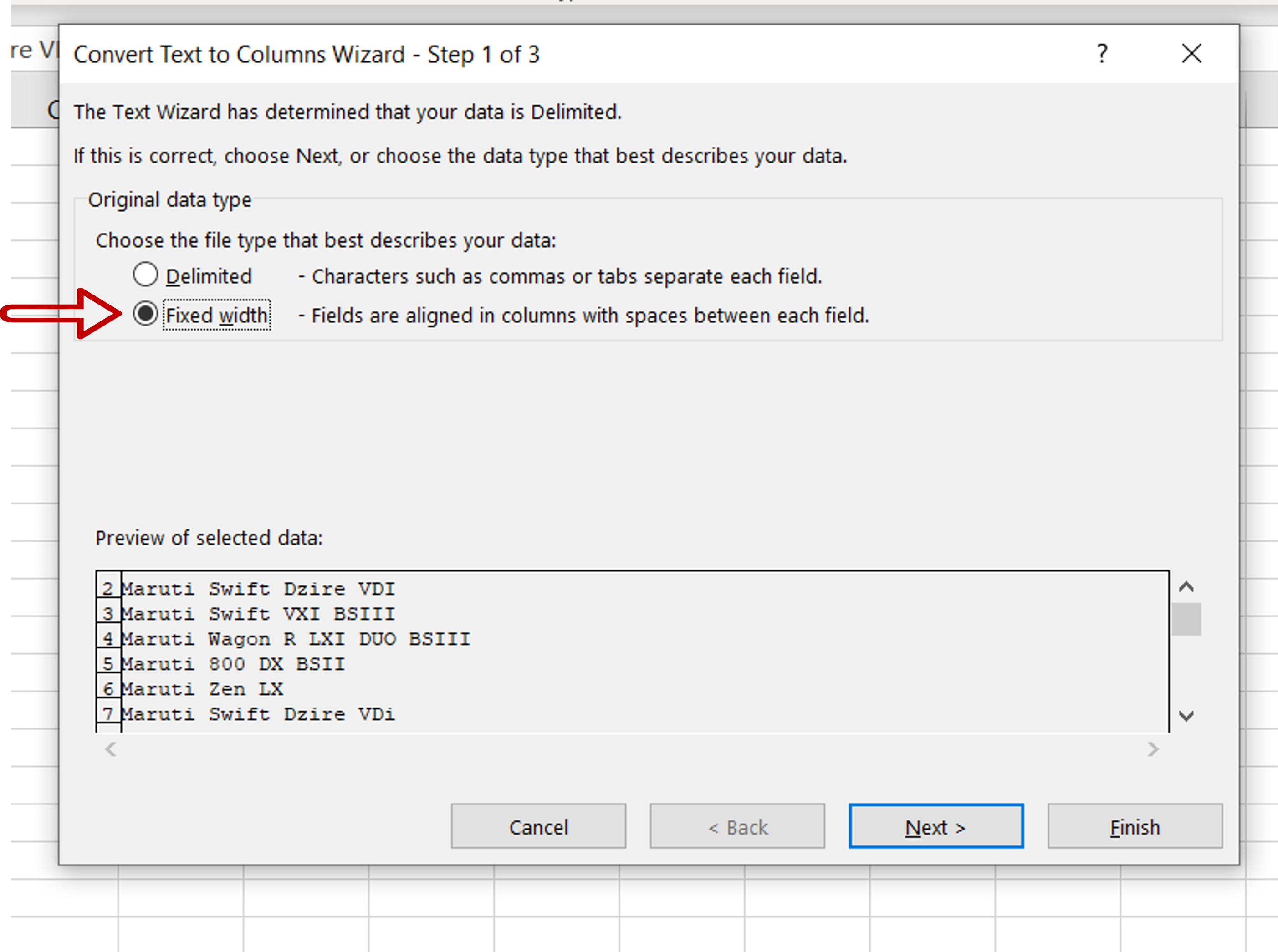
– Select the Fixed width option
– Click on Next
Step 3 – Check the preview
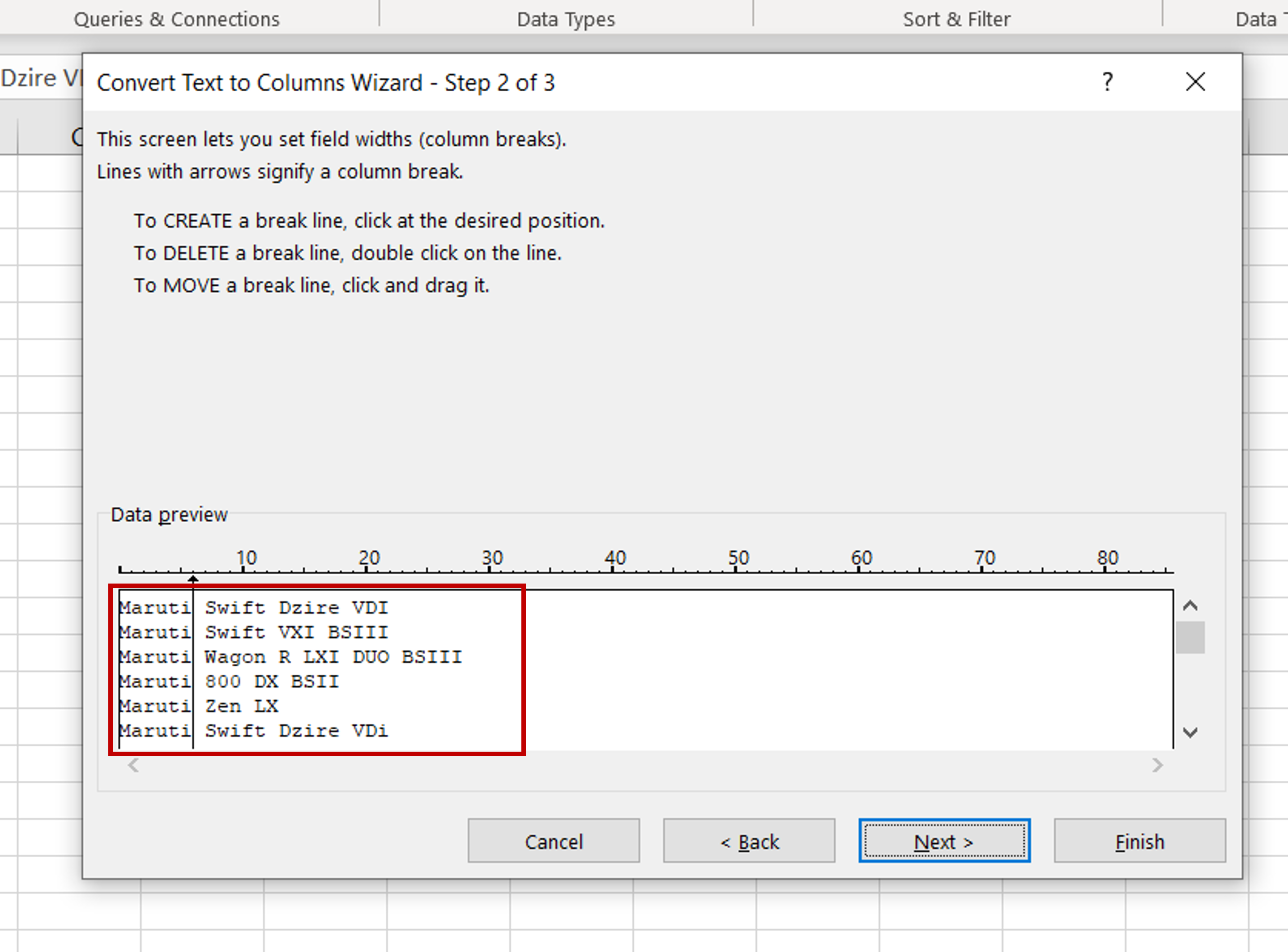
– Check that the data has been separated correctly in the Data preview
– Click Next
Step 4 – Choose the format and destination
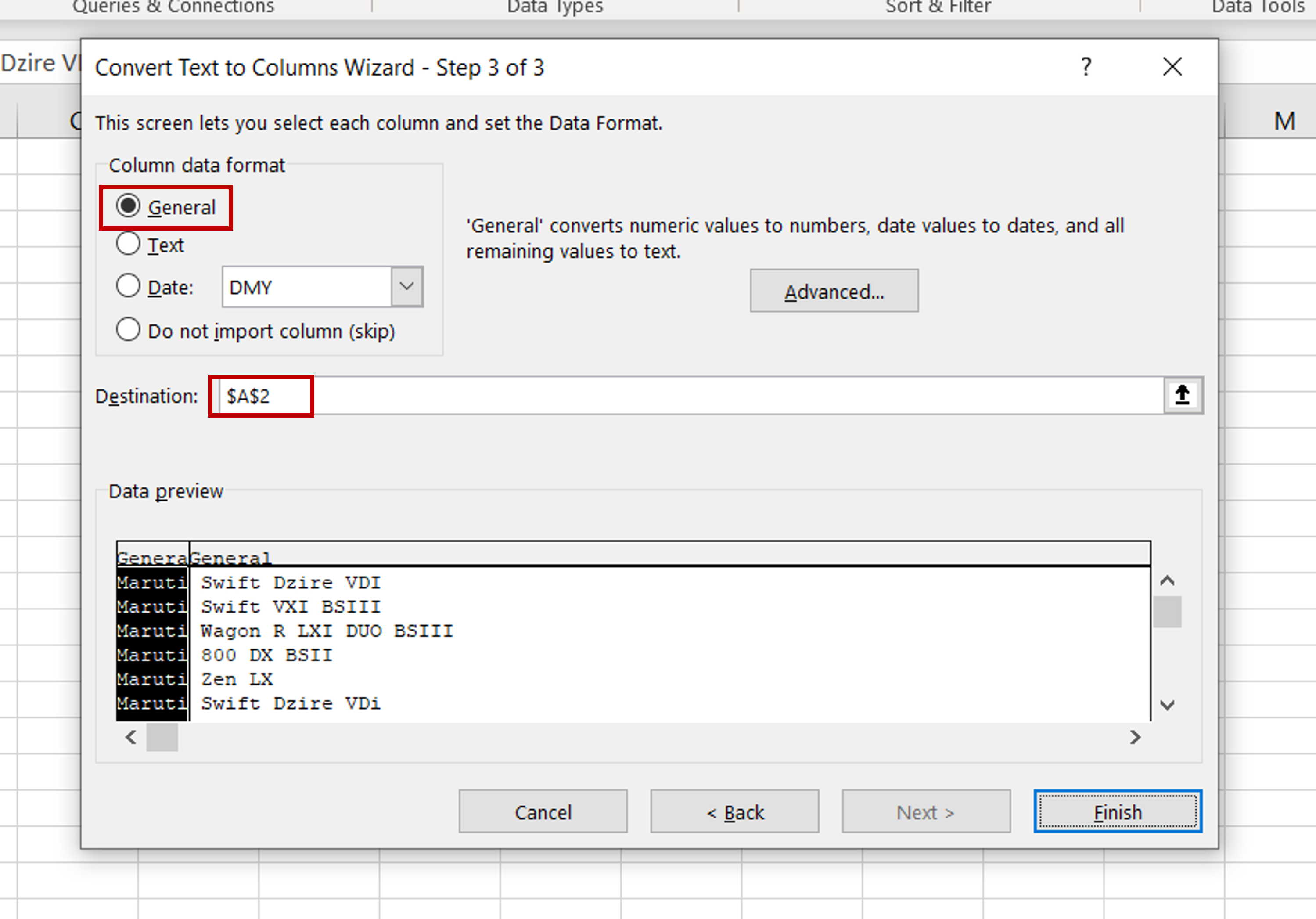
– Under Column data format, choose General
– Select the Destination for the data
– Click Finish
Step 5 – Sort the remaining data
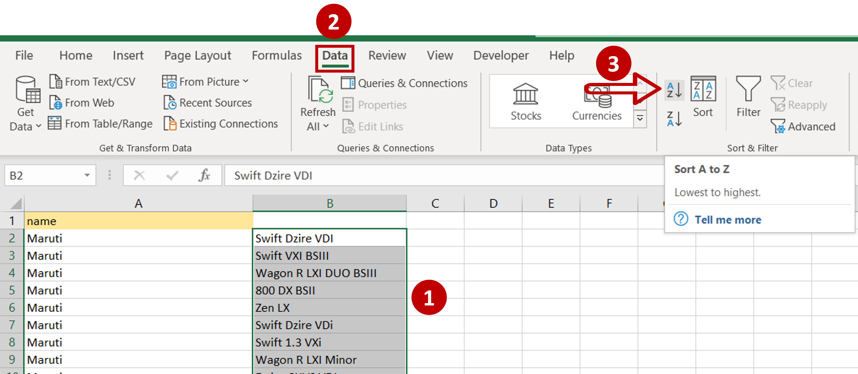
– The manufacturer’s name is separated from the rest of the data
– Select the column with the rest of the data
– Go to Data > Sort & Filter
– Click on the Sort A to Z button
– In the Sort warning box select Continue with the current selection
– Click Sort
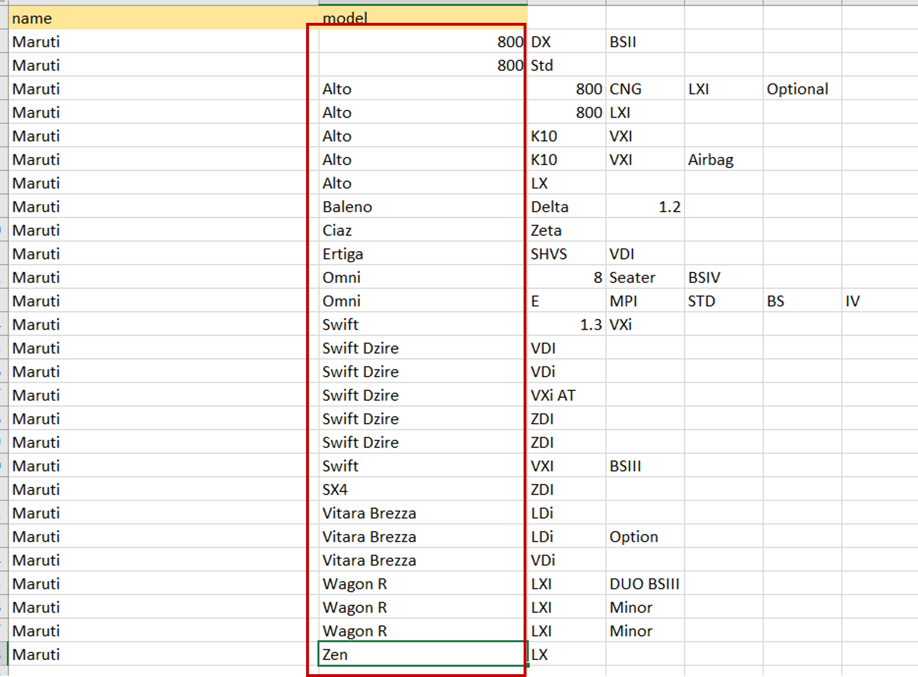
Step 6 – Select the next set of data
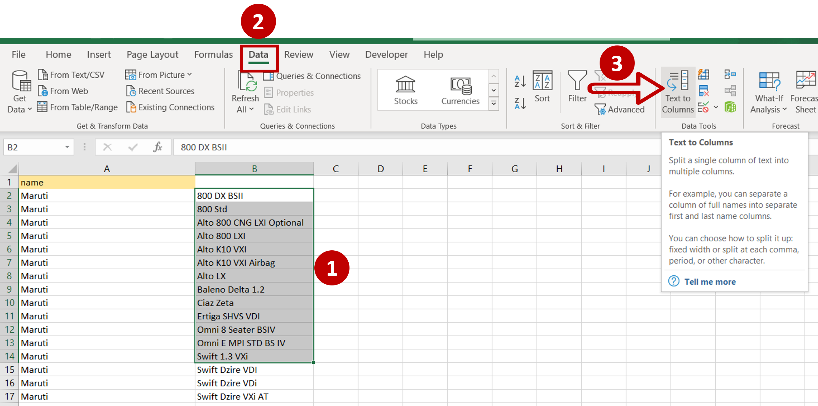
– Select the next set of data that can be separated based on a space delimiter
– Go to Data > Data Tools
– Click on Text to Columns
Step 7 – Choose the file type
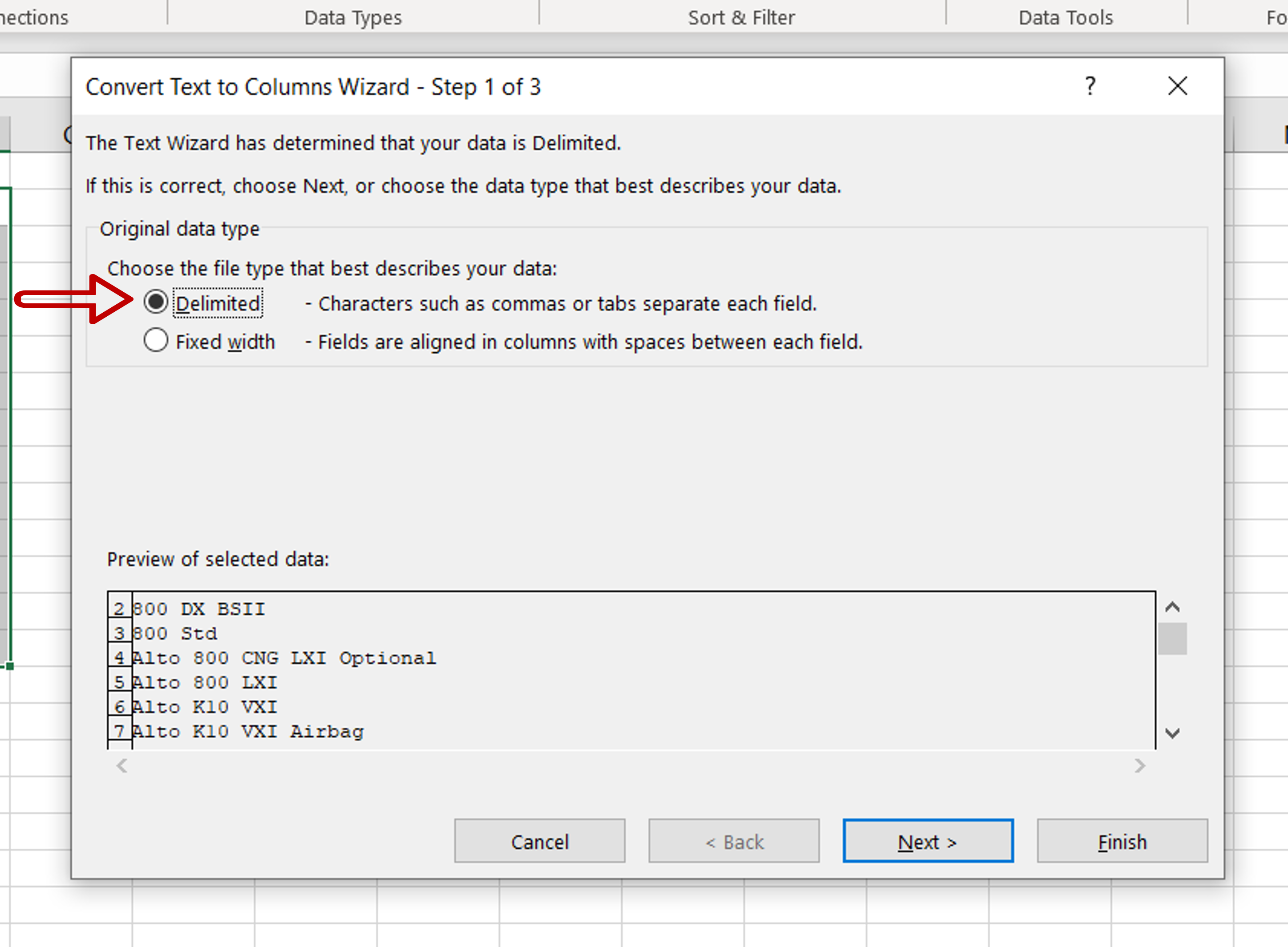
– Select the Delimited option
– Click on Next
Step 8 – Choose the delimiter
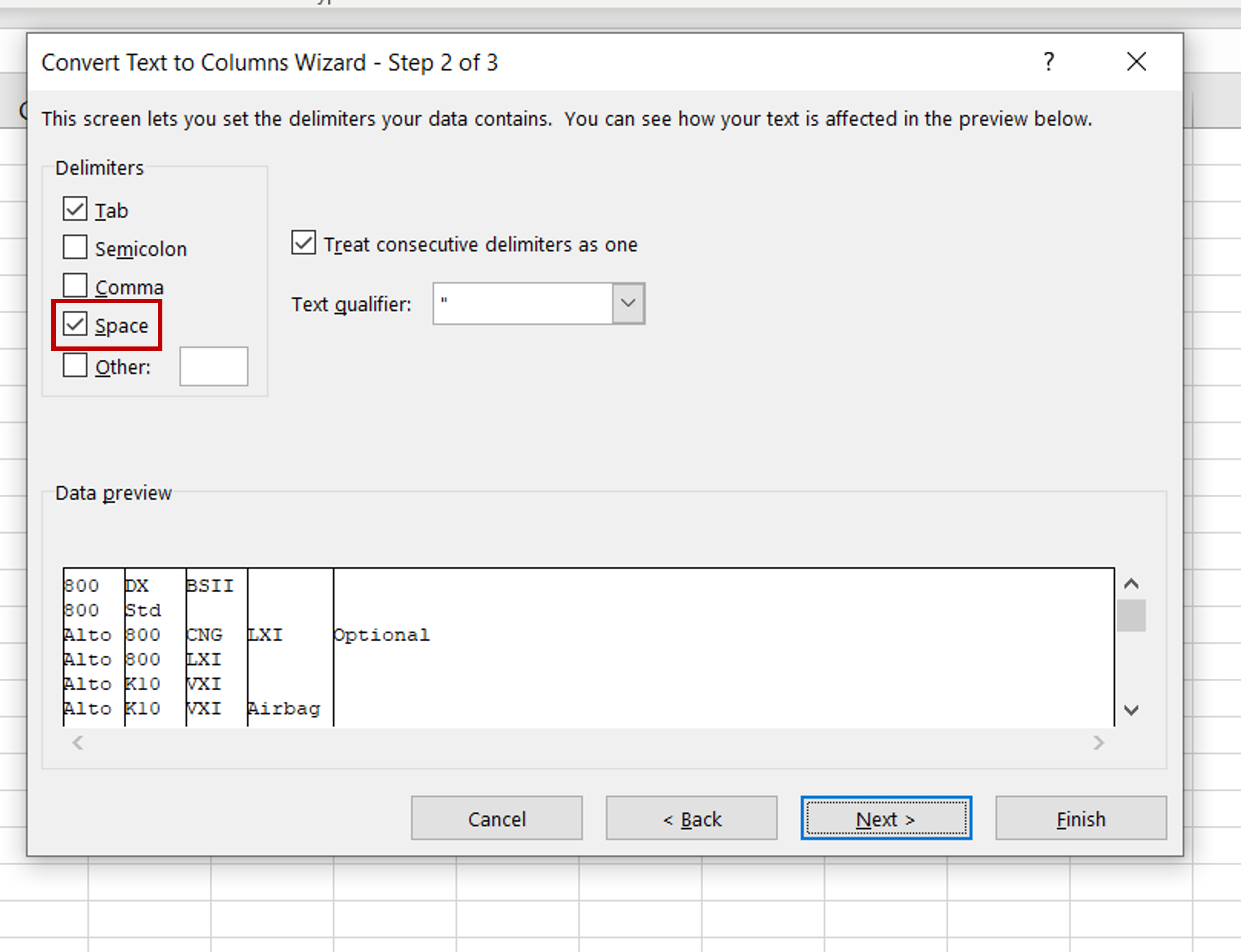
– Choose Space as the delimiter
– Check that the data has been separated correctly in the Data preview
– Click Finish
Step 9 – Separate the rest of the data
– Separate the rest of the column using the Text to Columns wizard with either the Delimited or Fixed width option
– Delete the unwanted columns


