How to select rows with specific text in Microsoft Excel 

In Microsoft Excel, selecting rows with specific text means selecting only those rows in a worksheet that contain a certain piece of text. This is useful when you want to filter or analyze data based on specific criteria. Once you have filtered your data to show only the rows that contain the specific text you are interested in, you can perform further analysis or calculations on the filtered data.

In this tutorial, we will learn how to select rows with specific text in Microsoft Excel. Selecting rows that contain specific text is a crucial task in Excel that can be accomplished through various methods. For instance, you can use the built-in filter feature or the Find & Select option available in the Home tab. Additionally, conditional formatting can also be utilized to highlight or select rows that contain specific text.

Currently, we have a data set representing the details of employees of a company. We want to select the details of the Marketing department only.

Method 1: Using the Filter Feature 

Step 1 – Select the Data

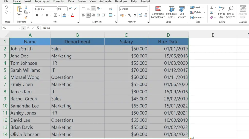
• Select the data containing the rows with specific text.

Step 2 – Click on the Sort & Filter Button

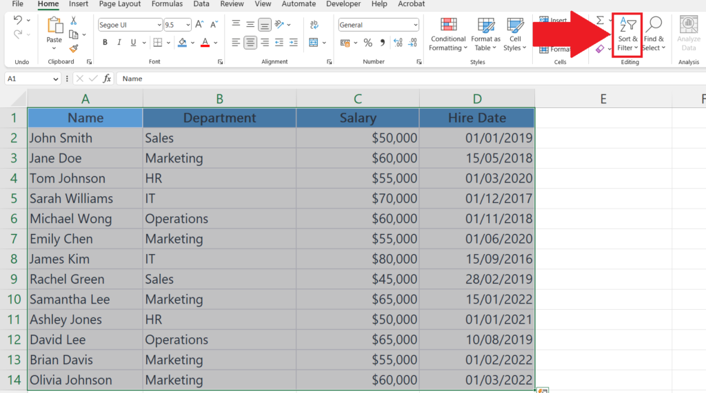
• Click on the Sort & Filter button in the Editing section of the Home tab.
• Filter drop-down arrows will appear next to the header of each column.

Step 3 – Click on the Sort Option

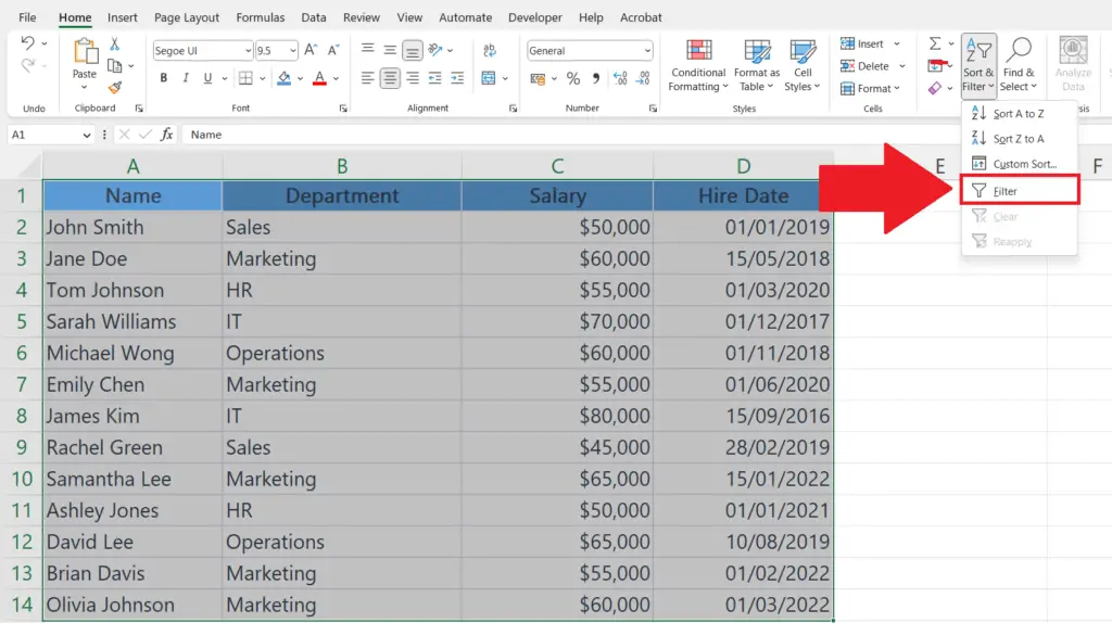
• Click on the Sort option in the drop-down menu.

Step 4 – Click on the Filter Drop-down Arrow 

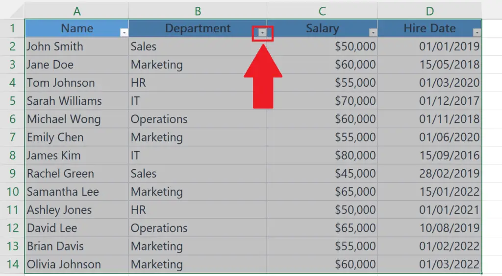
• Click on the Filter drop-down arrow of the column containing the specific text.

Step 5 – Click on the Text Filters Option

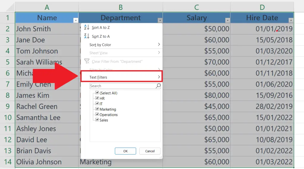
• Click on the Text Filters option in the filter drop-down list.

Step 6 – Click on Contains Option

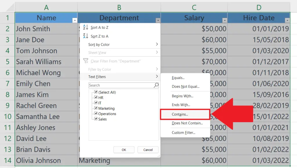
• Click on the Contains option.
• The Custom Autofilter dialog box will appear.

Step 7 – Enter the Specific Text and Click on OK

• Enter the specific text in the option next to contains.
• Click on OK in the Custom Autofilter dialog box.
• Only the rows containing the specified text will be displayed.

Step 8 – Now Select All the Rows

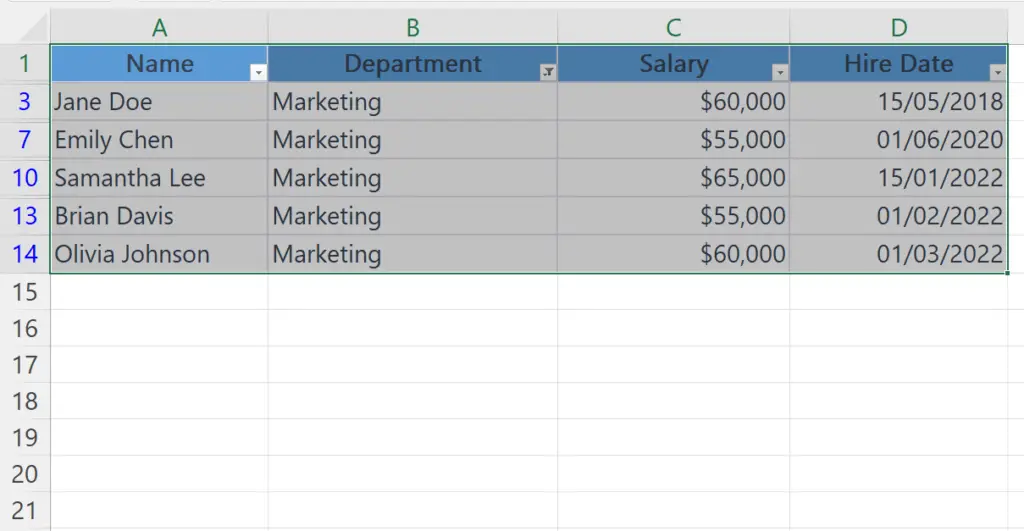
• Now select all the rows.
• You may use the “Handle Select” and “Drag and Drop” methods or CTRL + A shortcut keys.

Method 2: Using the Find & Select Feature

Step 1 – Press CTRL + F Shortcut Keys

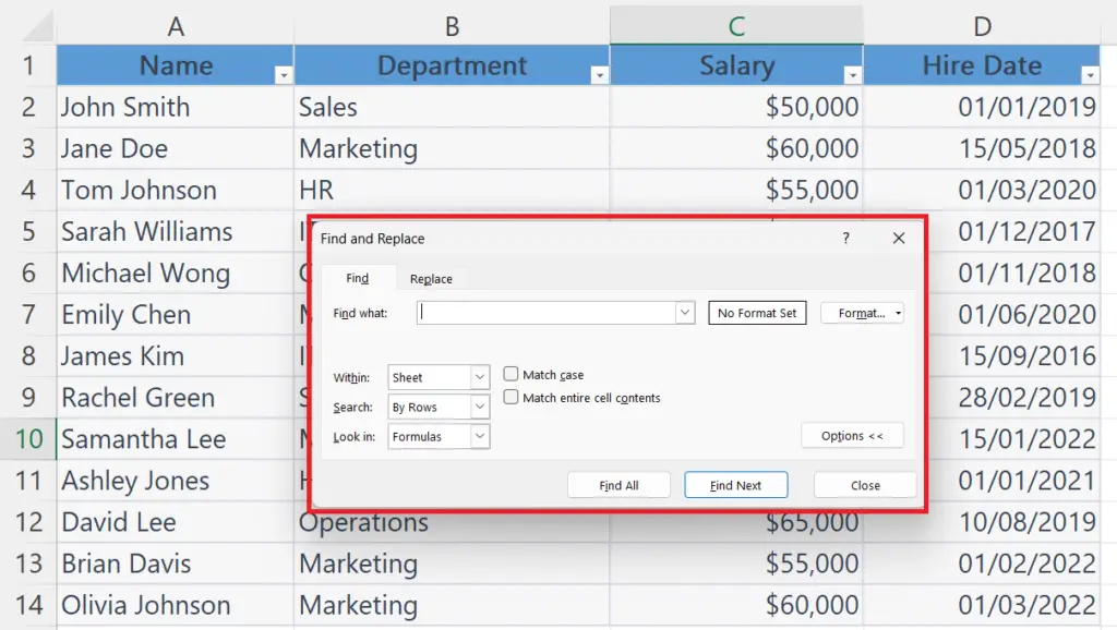
• Press CTRL + F shortcut keys to open the Find and Replace dialog box.

Step 2 – Enter the Specific Text

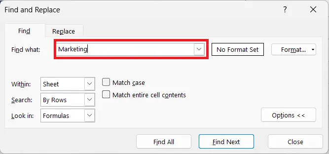
• Enter the specific text in the Find option, based on which you want to select the rows.

Step 3 – Click on the Find All Option

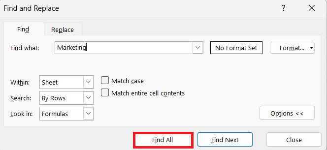
• Click on the Find All option.
• All the cells containing the text would be listed.

Step 4 – Select All the Cells and Click on Close

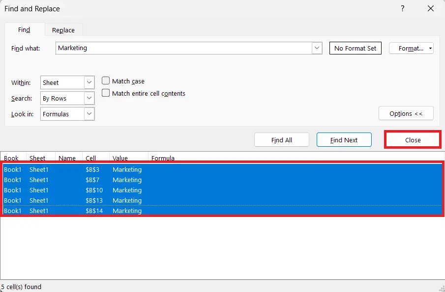
• Select all the listed cells.
• Click on the close option in the Find and Replace dialog box.

Step 5 – Press CTRL Key and Select the Rows

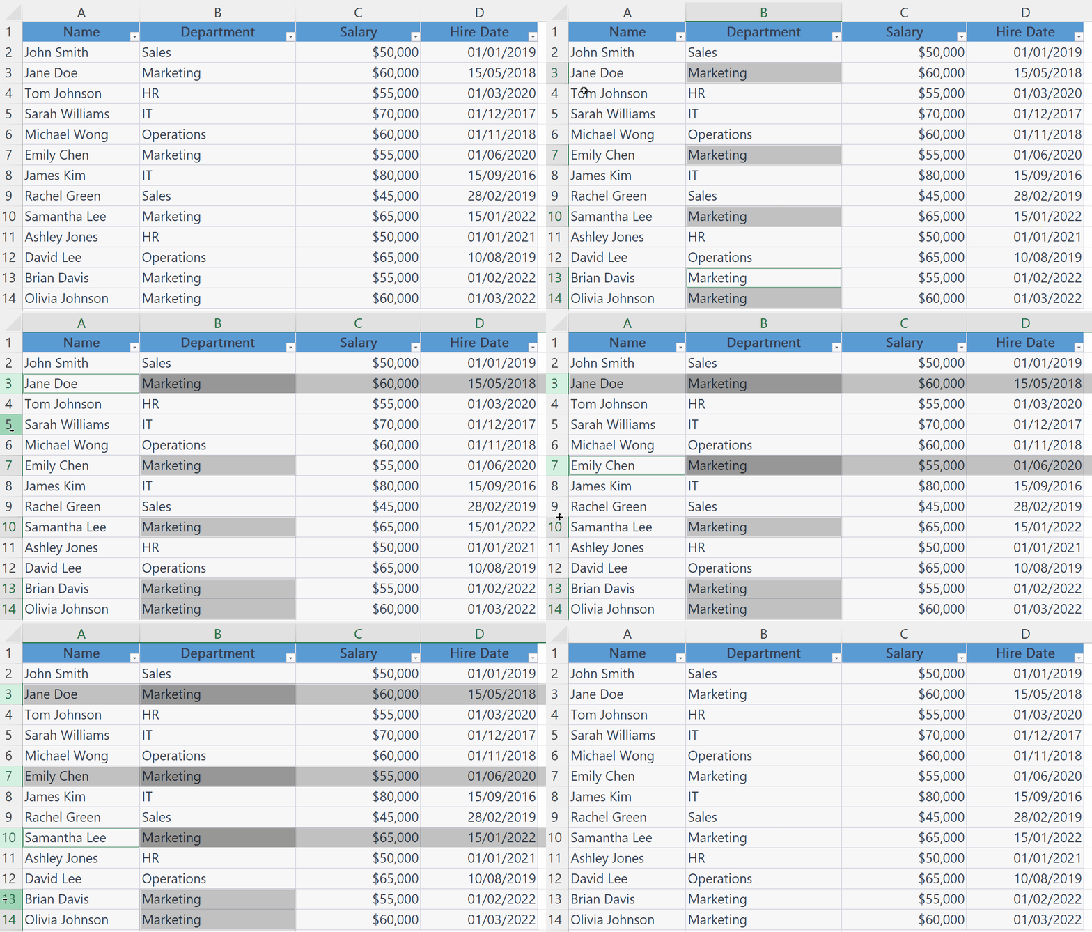
• Press the CTRL key and select all the rows of selected cells by clicking the row headers.

Method 3: Using the Conditional Formatting

Step 1 – Select the Data

• Select the data containing the rows with specific text.

Step 2 – Click on the Conditional Formatting Button

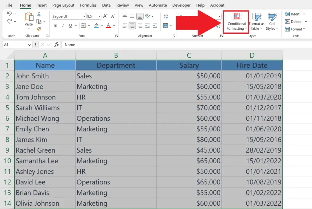
• Click on the Conditional Formatting button in the Styles section in the Home tab.

Step 3 – Click on the New Rule Option

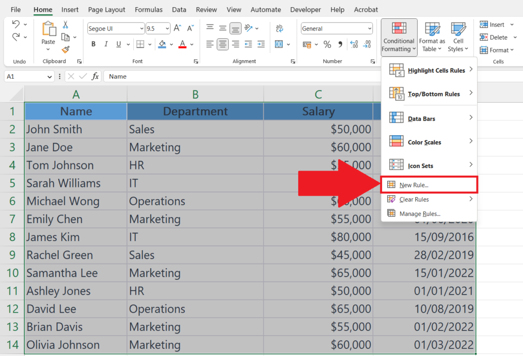
• Click on the New Rule option in the drop-down menu.

Step 4 – Select “Format only cells that contain” Option

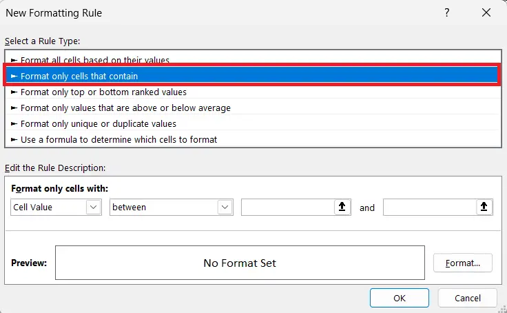
• Select the “Format only cells that contain” option in the “Select a Rule Type” option.

Step 5 – Click on the List Arrow of the “Format Only Cells With” Option

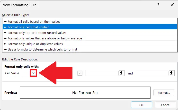
• Click on the First List Arrow of the “Format Only Cells With” Option.

Step 6 – Select Specific Text Option

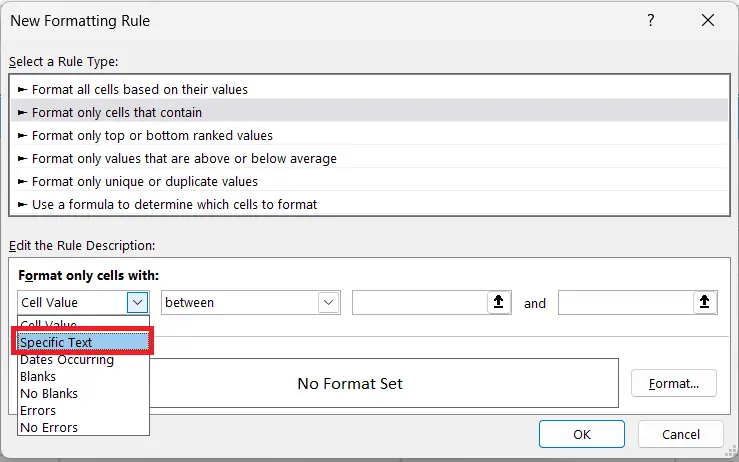
• Select the Specific Text option in the list.

Step 7 – Click on the Format Button and Select a Fill Colour

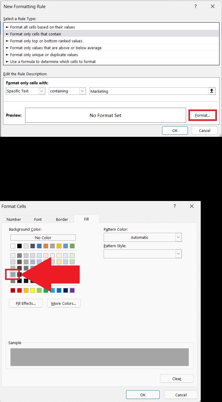
• Click on the Format button and Select a Fill Colour.

Step 8 – Click on OK 

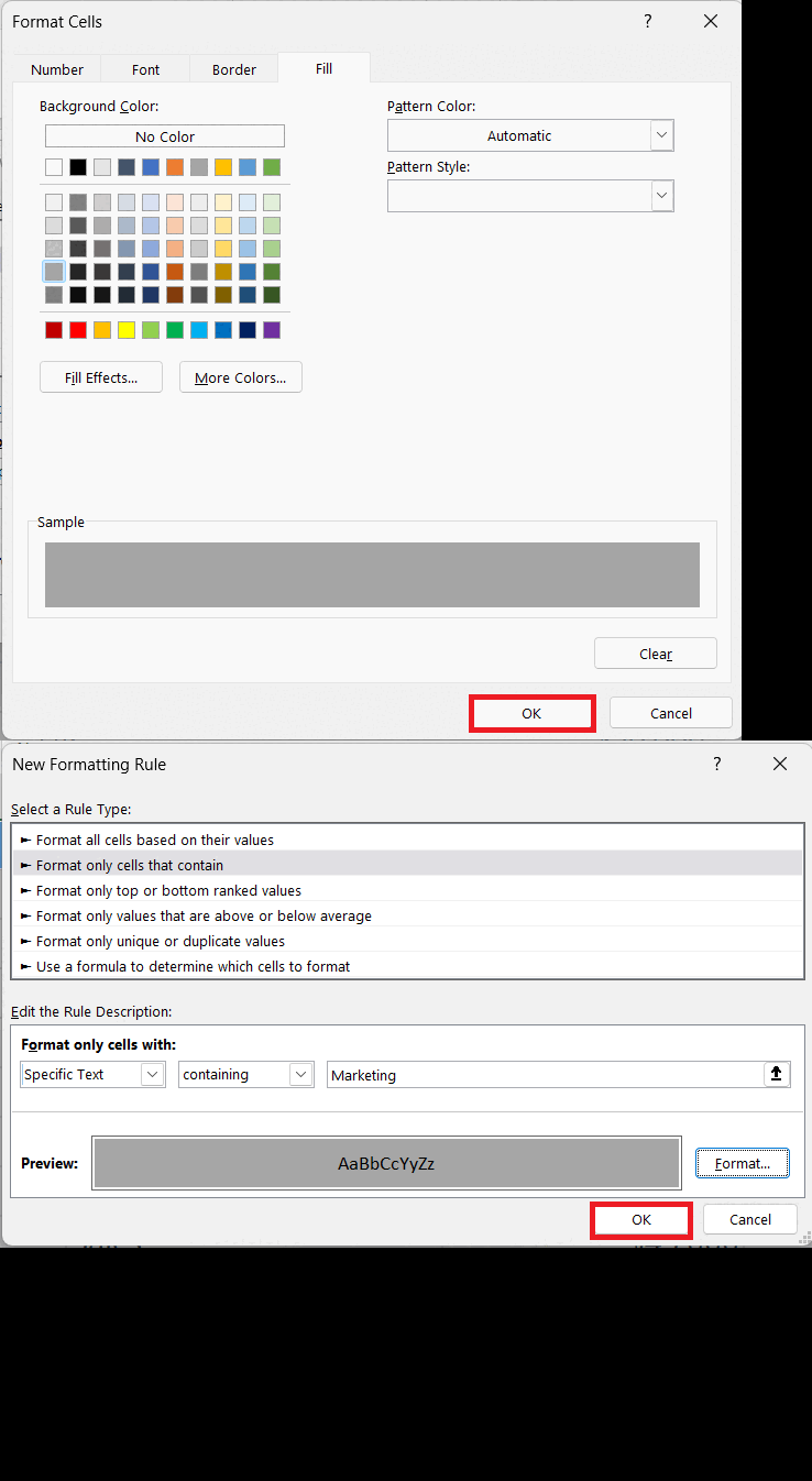
• Click on OK in the Format Cells dialogue box.
• Click on OK in the New Formatting Rule dialogue box.
• All the Cells with the specified text would be highlighted.

Step 9 – Press CTRL Key and Select the Rows

• Select all the rows containing the specific text by holding the CTRL key and clicking on the row headers.