How to select a random sample in Excel

You can watch a video tutorial here.

Excel can be used to select a random sample from a set of data. Random sampling is a method used often in statistical analysis. Suppose you have 200 students that take a class and you are interested in knowing their feedback about the class. You decide to interview the students but interviewing 200 students is too big a task. You decide instead to interview only a sample of 30 students with the confidence that this will give you a good idea of the opinion of the entire class. The problem now arises of how to select the 30 students. This is where random sampling can be used to pick 30 students at random from the list. In Excel, there are 2 ways in which this can be done:

1. Using the Data Analysis tool
2. Using the RAND() function: this returns a random number
   1. Syntax: RAND()

Option 1 – Use the Data Analysis tool

Note: If the Data Analysis button is present under Data > Analyze,  then skip steps 1 to 3

Step 1 – Open the Excel Options window

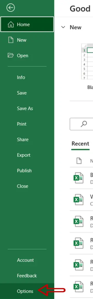
• Go to File > Options

Step 2 – Manage the Add-ins

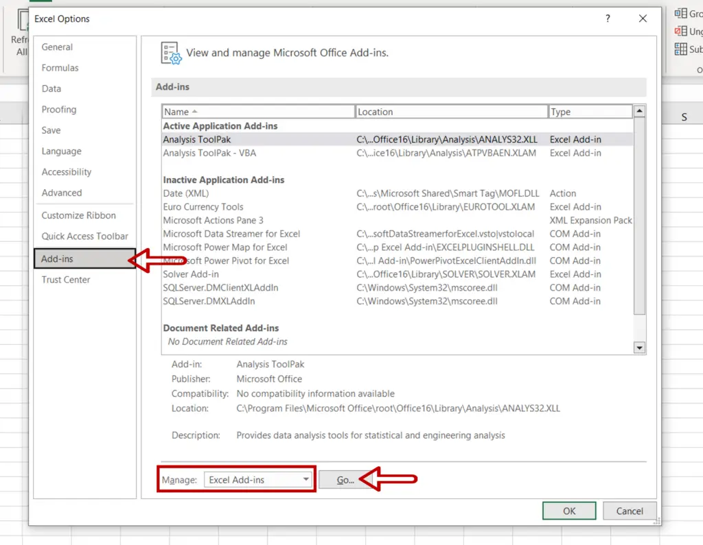
• Go to Add-ins
• Select Excel Add-ins from the Manage drop-down
• Click Go

Step 3 – Load the Analysis ToolPak add-in

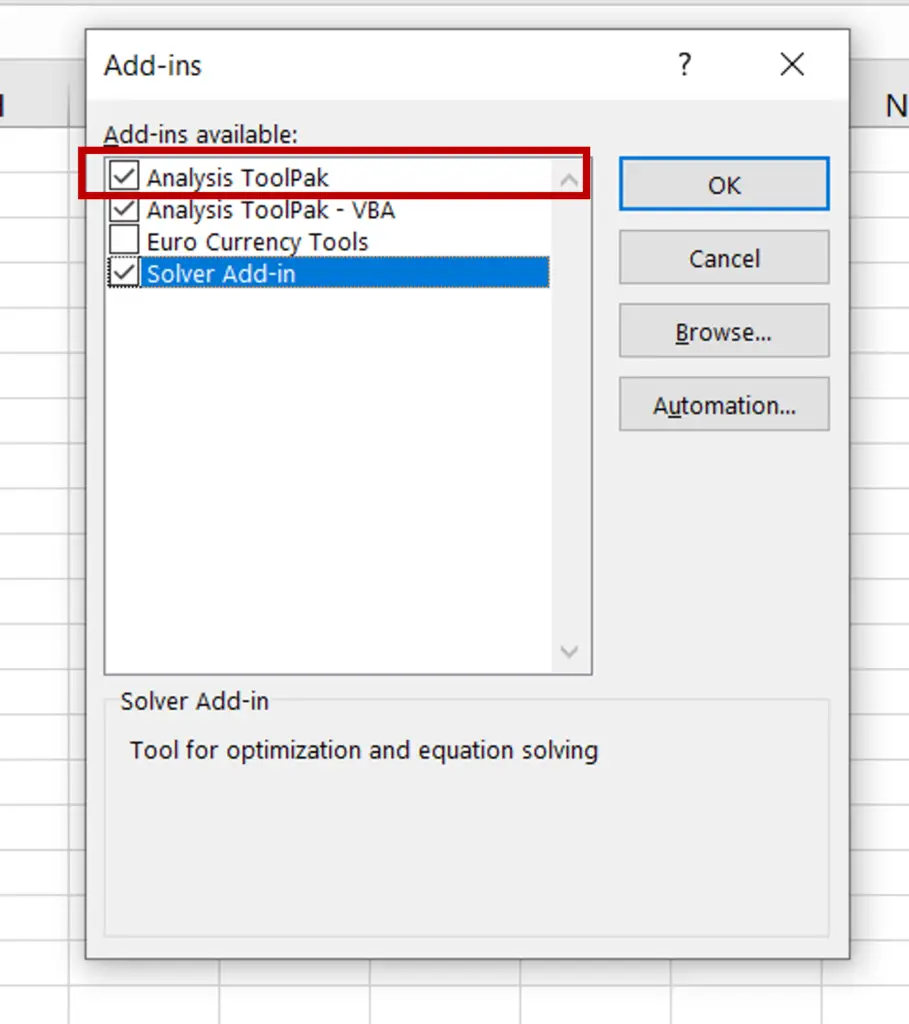
• Select Analysis ToolPak
• Click OK

Step 4 – Open the Data Analysis box

• Go to Data > Analyze
• Click on Data Analysis

Step 5 – Open the Sampling box

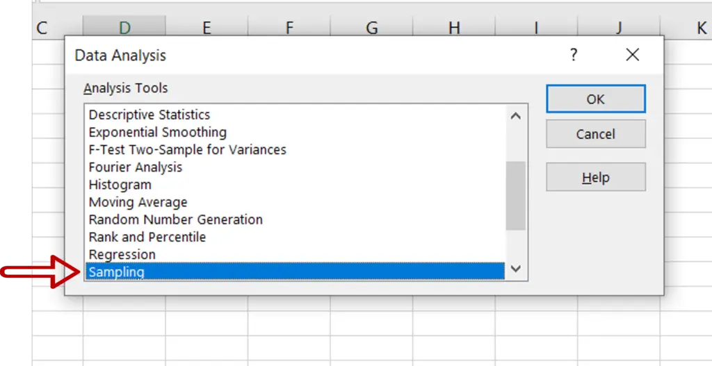
• Select Sampling
• Click OK

Step 6 – Set the parameters

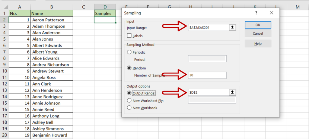
• Set the parameters as follows:
  • Input range: the range of the ‘No.’ column
  • Sampling Method: random
    • Number of Samples: 30
  • Output range: a location on the same sheet

Note: This method accepts only numeric data so the ‘No.’ column is used

• Click OK

Step 7 – Create a formula for the names

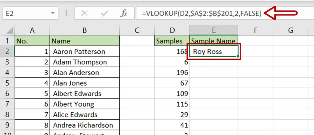
• A list of 30 random numbers is extracted from the list
• Select the cell next to the first number in the list
• Type the formula using cell references:

=VLOOKUP(Sample, $range of the list of names$,2,FALSE)

Note: The Vlookup formula looks for a value in a list and returns a value from the same row. The range is made constant so that the formula can be copied.

Step 8 – Copy the formula

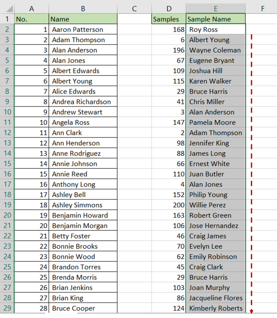
• Using the fill handle from the first cell, drag the formula to the remaining cells

OR

1. Select the cell with the formula and press Ctrl+C or choose Copy from the context menu (right-click)
2. Select the rest of the cells in the column and press Ctrl+V or choose Paste from the context menu (right-click)

• The list of random samples is created

Option 2 – Use the RAND() function

Step 1 – Create the formula

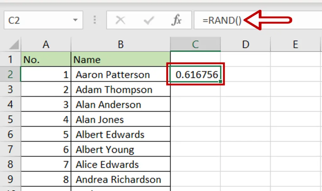
• Select the cell next to the first name
• Enter the function and press Enter:

=RAND()

Step 2 – Copy the formula

• A random number will be generated
• Using the fill handle from the first cell, drag the formula to the remaining cells

OR

1. Select the cell with the formula and press Ctrl+C or choose Copy from the context menu (right-click)
2. Select the rest of the cells in the column and press Ctrl+V or choose Paste from the context menu (right-click)

Step 3 – Open the Sort box

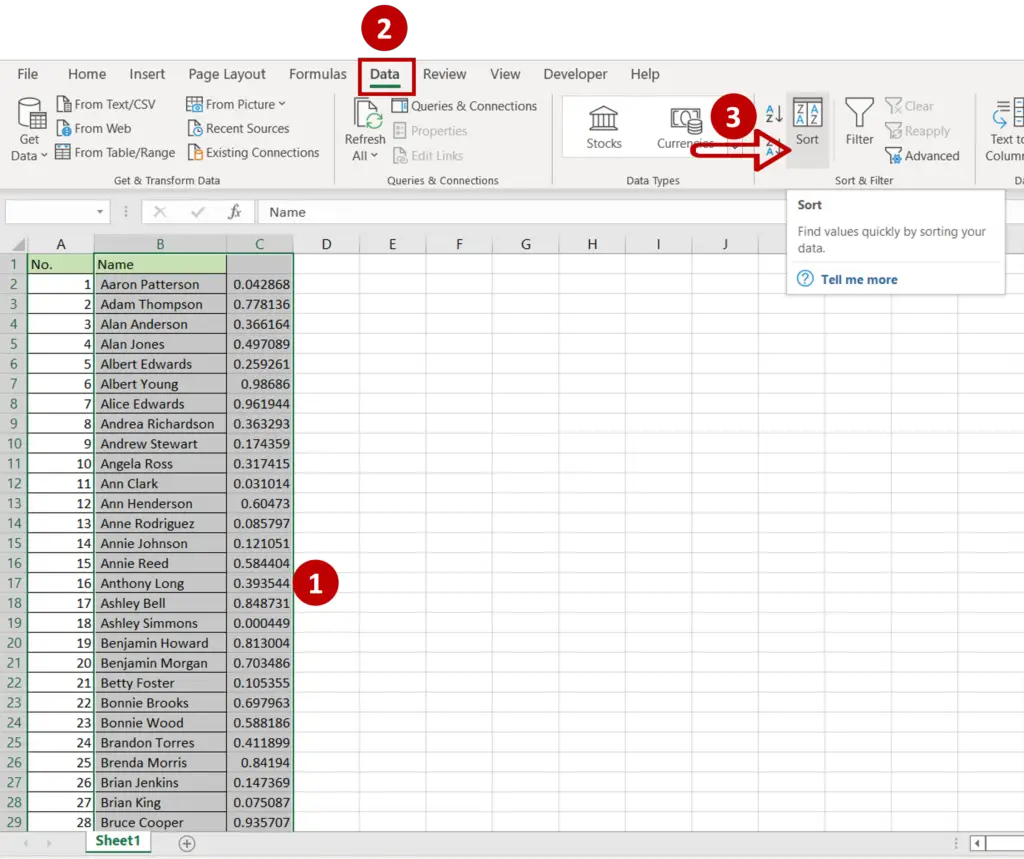
• Select the ‘Name’ column and the column with the random numbers
• Go to Data > Sort & Filter
• Click Sort

Step 4 – Set the parameters

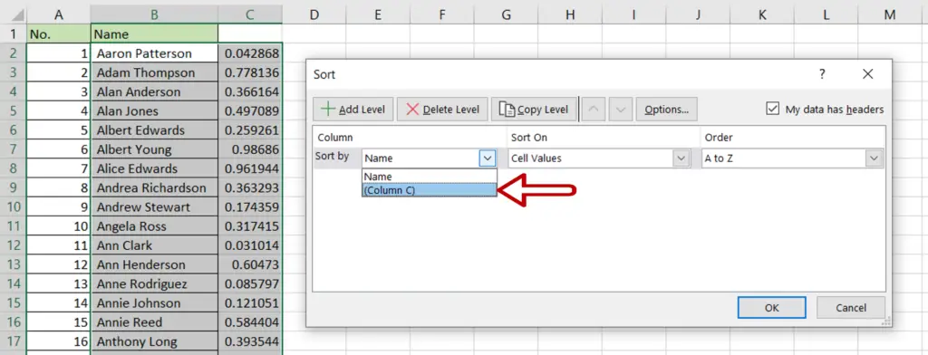
• Select the column with the random numbers from the list for Sort by
• Click OK

Step 5 – Select the random sample

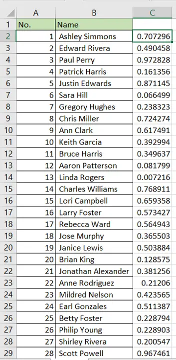
• The first 30 records serve as the random sample