How to search for multiple values in Excel

In this tutorial we will learn how to search for multiple values in excel. In our dataset information of students are present and in the same sheet we want a certain type of data only against the name of students. For this we used INDEX and MATCH functions.Following steps guides to use INDEX and MATCH functions.

Syntax of INDEX function

INDEX(array, row_num, [column_num])

• array: This is the range or array of cells that you want to return a value from. This argument is required.
• row_num: This is the row number within the array that you want to return a value from. This argument is required.
• column_num: This is the optional column number within the array that you want to return a value from.

Syntax of MATCH function

MATCH(lookup_value, lookup_array, [match_type])

• lookup_value: This is the value you want to find within the lookup array. This argument is required.
• lookup_array: This is the range or array of cells that you want to search for the lookup value. This argument is required
• match_type: This is an optional argument that specifies the type of match you want to perform. It can be set to 0, 1, or -1, depending on the type of match you want to perform. If omitted, the function will default to a value of 1.

When you search for multiple values in Excel, you are looking for data that matches any of a set of specified criteria. For example, you may have a large dataset with multiple columns of data, and you want to find all the rows that contain any of a list of specific values in one of those columns. This is often useful when you want to analyze or work with a subset of the data that meets certain criteria. It makes working on excel efficient and has less chance of error.

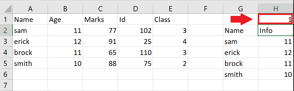
Step 1 – select the cell

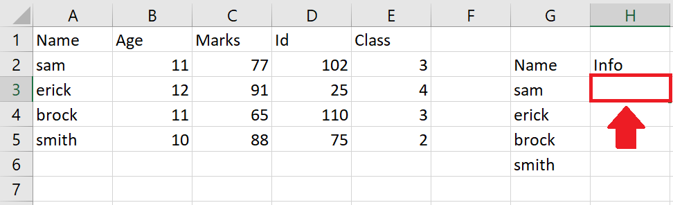
– Select the cell where you want to show the data

Step 2 – Type Formula

– Type the following formula in selected cell 
=INDEX(B2:E5, MATCH(G3:G6,A2:A5,0),H1)

Step 3 – Type the column number

– Type the column numbers in the cell H1 (selected as column-num) to get different types of data from the source data and press enter key to get the required result as shown above.

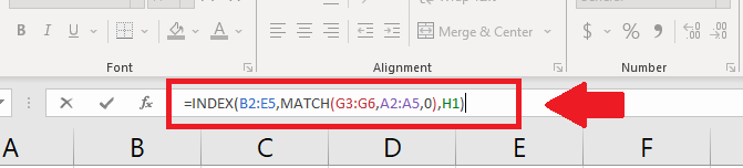
Explanation of the formula used

=INDEX(B2:E5, MATCH(G3:G6,A2:A5,0),H1)

• The MATCH function searches for the value in cell G3 within the range A2:A5, and returns the position of the first cell in the range that contains an exact match. The 0 argument tells the function to look for an exact match. 
• The INDEX function uses the position returned by MATCH to return the value in the same row and the column specified by the value in cell H1. The range B2:E5 is used as the array from which to return the value. 
• So, the formula returns a single value from the range B2:E5 based on the position of the lookup value in G3 and the column specified in H1.