
How to round to the nearest hundred in Excel
 By
SpreadCheaters
By
SpreadCheaters
You can watch a video tutorial here.
Excel is frequently used for calculations and has many functions to help with basic mathematical operations. There are several functions and formatting options available to round numbers up or down. When a number has decimal places, the number can be rounded off using formatting or by using a function. You may have a number that does not have decimal places but you want to round it to the nearest hundred so that it is easier for the reader to understand. For example, when comparing sales figures across branches, rounding the numbers to the nearest hundred makes it easier to compare the numbers.
In Excel, you can use any one of the functions described below. These ROUND, ROUNDUP and ROUNDDOWN functions use positive numbers to round off decimal places. To round numbers to the left of the decimal point, negative numbers are used.
- ROUND(): this rounds the number up or down to the specified number of digits
- Syntax: ROUND(number, num_digits)
- number: the number to be rounded
- num_digits: the number of decimal places to which the number is to be rounded
- Syntax: ROUND(number, num_digits)
- ROUNDUP(): this rounds the number up to the specified number of digits
- Syntax: ROUNDUP(number, num_digits)
- number: the number to be rounded
- num_digits: the number of decimal places to which the number is to be rounded
- Syntax: ROUNDUP(number, num_digits)
- ROUNDDOWN(): this rounds the number down to the specified number of digits
- Syntax: ROUNDDOWN(number, num_digits)
- number: the number to be rounded
- num_digits: the number of decimal places to which the number is to be rounded
- Syntax: ROUNDDOWN(number, num_digits)
- MROUND()
- Syntax: MROUND (number, multiple)
- number: this is the number to be rounded
- multiple: the multiple to which the number is to be rounded
- Syntax: MROUND (number, multiple)
Option 1 – Use the ROUND() function
Step 1 – Create the formula
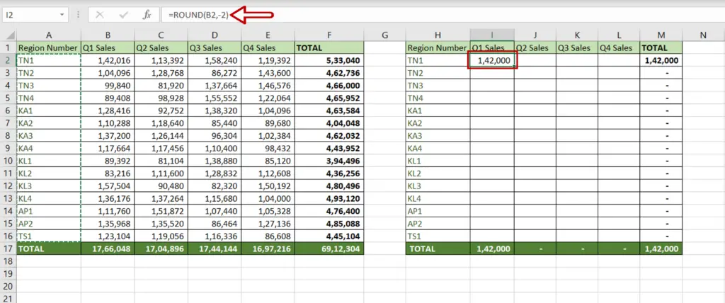
- Select the destination cell
- Type the formula using cell references:
=ROUND(Q1 Sales,-2)
- Press Enter
Step 2 – Copy the formula
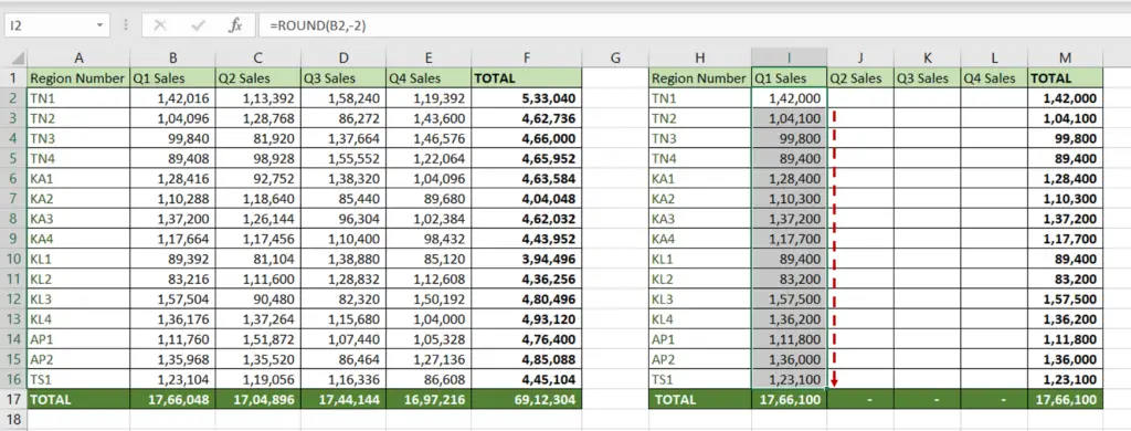
- Using the fill handle from the first cell, drag the formula to the remaining cells
OR
- Select the cell with the formula and press Ctrl+C or choose Copy from the context menu (right-click)
- Select the rest of the cells in the column and press Ctrl+V or choose Paste from the context menu (right-click)
- The numbers are rounded (either up or down, depending on the value of the number), to the nearest 100
Option 2 – Use the ROUNDUP() function
Step 1 – Create the formula
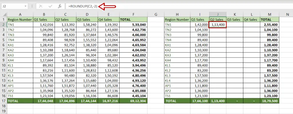
- Select the destination cell
- Type the formula using cell references:
=ROUNDUP(Q2 Sales,-2)
- Press Enter
Step 2 – Copy the formula
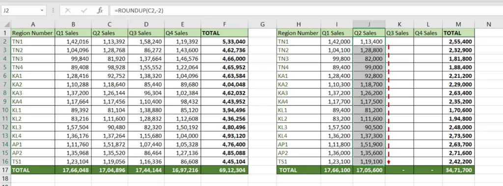
- Using the fill handle from the first cell, drag the formula to the remaining cells
OR
- Select the cell with the formula and press Ctrl+C or choose Copy from the context menu (right-click)
- Select the rest of the cells in the column and press Ctrl+V or choose Paste from the context menu (right-click)
- The numbers are rounded up to the nearest 100
Option 3 – Use the ROUNDDOWN() function
Step 1 – Create the formula
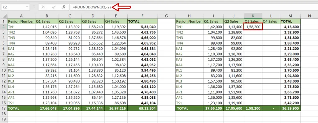
- Select the destination cell
- Type the formula using cell references:
=ROUNDDOWN(Q3 Sales,-2)
- Press Enter
Step 2 – Copy the formula
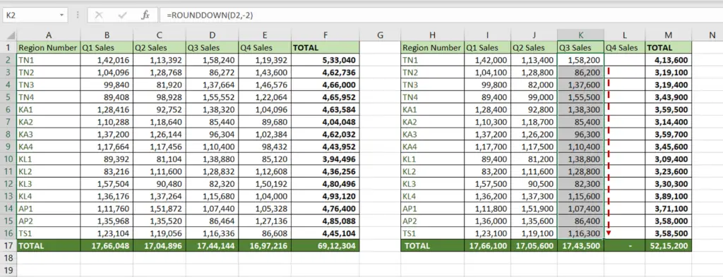
- Using the fill handle from the first cell, drag the formula to the remaining cells
OR
- Select the cell with the formula and press Ctrl+C or choose Copy from the context menu (right-click)
- Select the rest of the cells in the column and press Ctrl+V or choose Paste from the context menu (right-click)
- The numbers are rounded down to the nearest 100
Option 4 – Use the MROUND() function
Step 1 – Create the formula
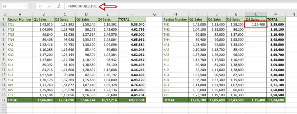
- Select the destination cell
- Type the formula using cell references:
=MROUND(Q4 Sales,100)
- Press Enter
Step 2 – Copy the formula
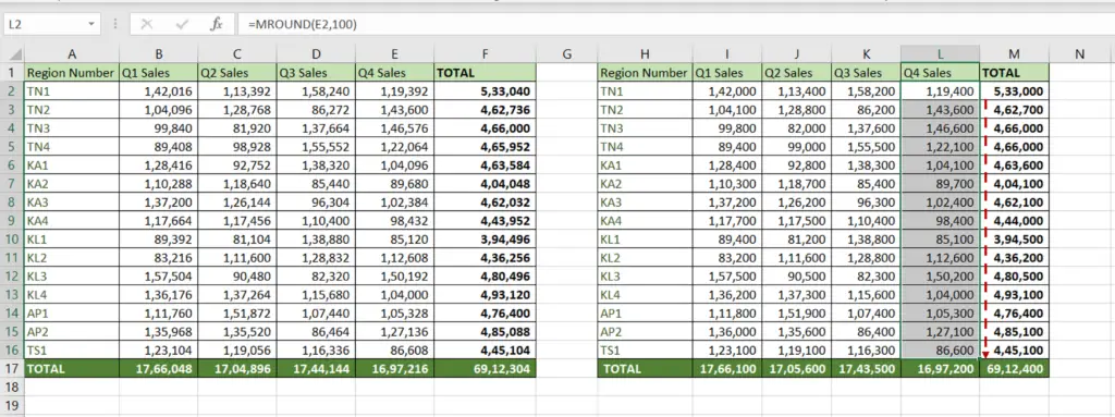
- Using the fill handle from the first cell, drag the formula to the remaining cells
OR
- Select the cell with the formula and press Ctrl+C or choose Copy from the context menu (right-click)
- Select the rest of the cells in the column and press Ctrl+V or choose Paste from the context menu (right-click)
- The numbers are rounded up or down to the nearest multiple of 100


