How to round to the nearest dollar in Excel

Rounding off dollars ensures that the figures are accurate and don’t contain decimals that can cause discrepancies in financial calculations. Rounding off dollars can help to maintain consistency in financial reports, especially when dealing with large datasets. In some cases, rounding off dollars is required for regulatory compliance. For example, financial statements prepared for tax purposes or for financial reporting purposes may need to comply with certain rounding rules.

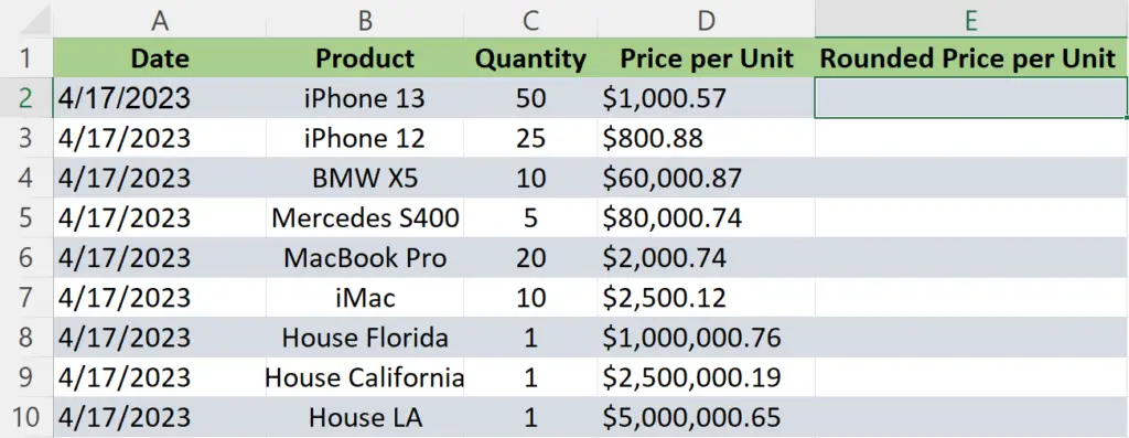
The following dataset contains information about sales of phones, cars, and houses in different states with sale rates in dollars with decimals. In today’s tutorial, we’ll learn how to round off the decimal of dollar values. Consider the following dataset as an example to understand today’s tutorial.

We’ll employ the following three methods to achieve this goal;

• Using the Decrease Decimal Action Button on the Home Tab
• The MROUND Function
• The CEILING Function

Follow the simple steps mentioned in different methods to round off:

Method 1 – Using Decrease Decimal Action Button

The easiest of all methods is to use the Home tab options. However, it is a manual method and you can control the amount of rounding off you need yourself by clicking on the decrease or increase decimal action button available on the Home Tab.

Step 1 – Copying all values to empty cells

• Select all cells of which you want to round values to the nearest dollar.
• Copy them by pressing Ctrl+C.
• Paste them in the new column by pressing Ctrl+V.

Step 2 – Using the Decimal Decrease action button

• After you have selected the copied cells, locate the decrease decimal option in the Home tab under the Number group.
• Click on the Decrease Decimal option until your dollar value is rounded to zero decimals.
• Now, all values are rounded to the nearest dollar.

Method 2 – Using the MROUND function

The MROUND function in Excel is a useful mathematical function that allows you to round a number to the nearest specified multiple. It is often used in financial calculations or when dealing with values that need to be rounded to specific increments. 

The syntax of the MROUND function is straightforward: =MROUND(number, multiple). 

Where;

number: This is the first argument that represents the value you want to round. 

multiple: The second argument specifies the increment or multiple of the number to which you want to round off the original number.

Step 1 – Writing the formula

• Select the cell in which you want to round off to the nearest dollar.
• Press the = button on the keyboard.
• Write MROUND and then press the tab to select the MROUND function.
• Then, enter the cell name that is to be rounded off e.g., D2
• After that, press the comma button, on your keyboard.
• Now, write 1 because we want to round to the nearest dollar.
• After doing this, close the parenthesis. The final formula should look like 

=MROUND(D2, 1)

• After that, press Enter and your value will be rounded to the nearest dollar.

Step 2 – Rounding off all values in column

• Select the cell in which the rounded off value is present
• Move your pointer to the bottom right corner of the cell until your pointer turns into + shape. 
• Drag down the cursor while pressing left-click.
• Now, all values of the column will be rounded off to the nearest dollar. 

Method 3 – Using the CEILING function

The CEILING function in Excel is a mathematical function that allows you to round a number up to the nearest specified multiple. It is commonly used in financial calculations or when dealing with values that need to be rounded up to specific increments.

The syntax of the CEILING function is simple: =CEILING(number, significance). 

Where;

number: This is the first argument and it represents the value you want to round up.

Significance: The second argument specifies the multiple you want to round up to.

Step 1 – Writing the formula

• Select the cell in which you want to round off to the nearest dollar.
• Press the = button on the keyboard.
• Write CEILING and then press the tab to select the CEILING function.
• Then, enter the cell name that is to be rounded off e.g., D2
• After that, press the comma button, on your keyboard.
• Now, write 1 because we want to round to the nearest dollar.
• After doing this, close the parenthesis and now the formula would look like 

=CEILING(D2, 1)

• After that, press Enter and your value will be rounded to the nearest dollar.

Step 2 – Rounding off all values in column

• Select the cell in which the rounded-off value is present
• Move your pointer to the bottom right corner of the cell until your pointer turns into + shape. 
• Drag down the cursor while pressing left-click.
• Now, all values of the column will be rounded off to the nearest dollar.