How to round Excel data to make summations correct

To make summations in Excel accurate, it is sometimes necessary to round the data by decreasing the number of decimal places in numerical values. By doing so, rounding errors resulting from the limitations of computer arithmetic can be prevented. 

In this tutorial, we will learn how to round Excel data to make summations correct. There are multiple ways to round data in Excel. One option is to use the Number format feature, another is to use the “Decrease Decimal” button, and a third option is to use functions such as ROUND and TRUNC.

Method 1: Utilizing the Number Format Option

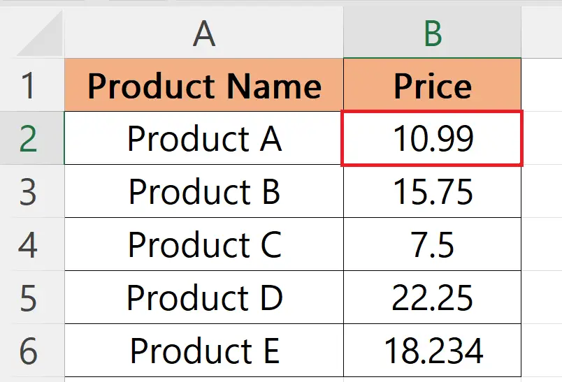
Step 1 – Choose the Cells

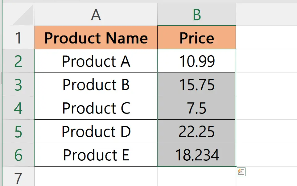
• Select the cells that hold the data you want to round.

Step 2 – Open the Format Cells Dialog Box

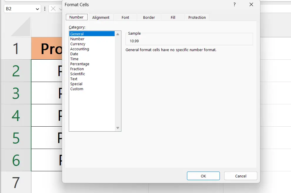
• Press the CTRL+1 keys to open the “Format Cells” dialog box.

Step 3 – Choose the Number Format 

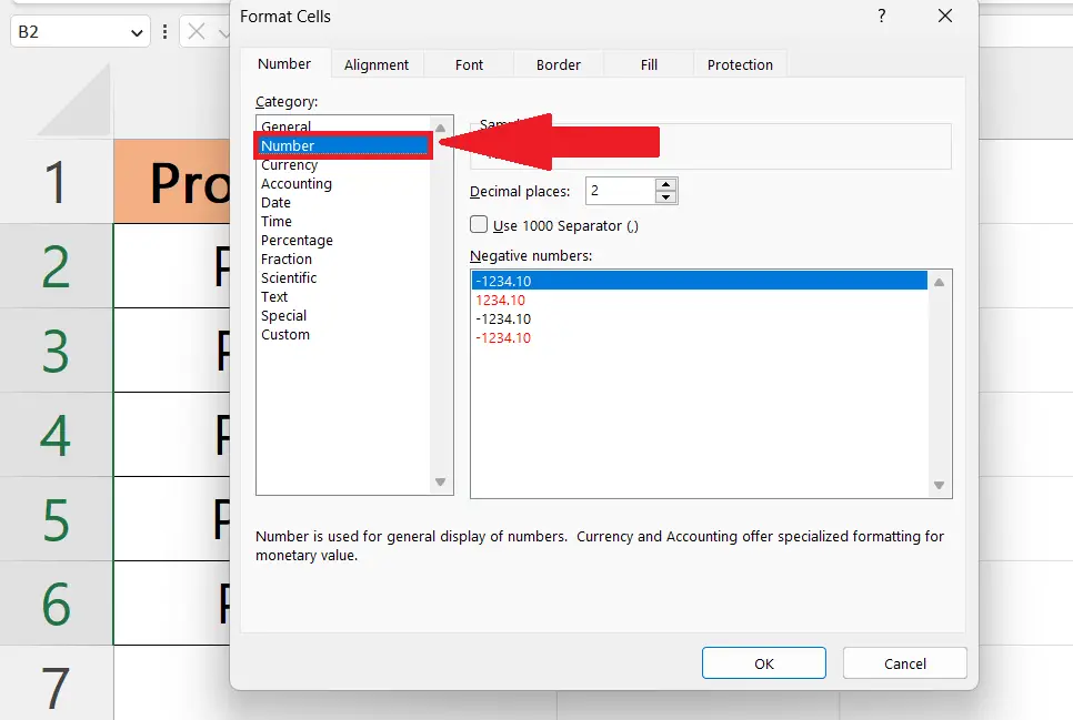
• Choose the Number format from the menu.

Step 4 – Set the Decimal Places to Zero and Hit the OK Button

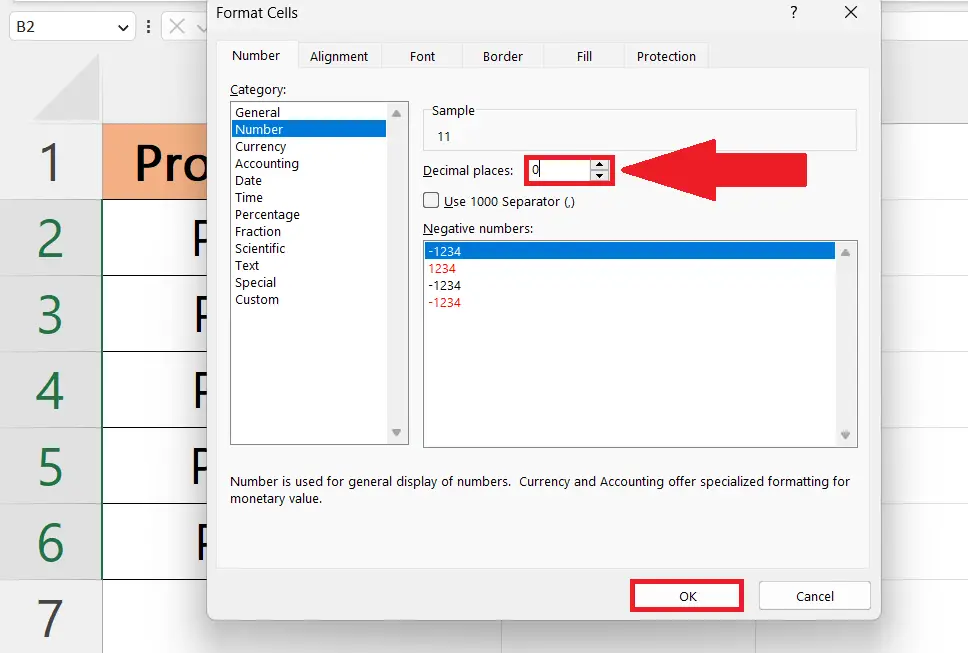
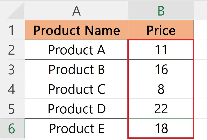
• Set the decimal places to zero and hit the OK button.
• The data will automatically be rounded.

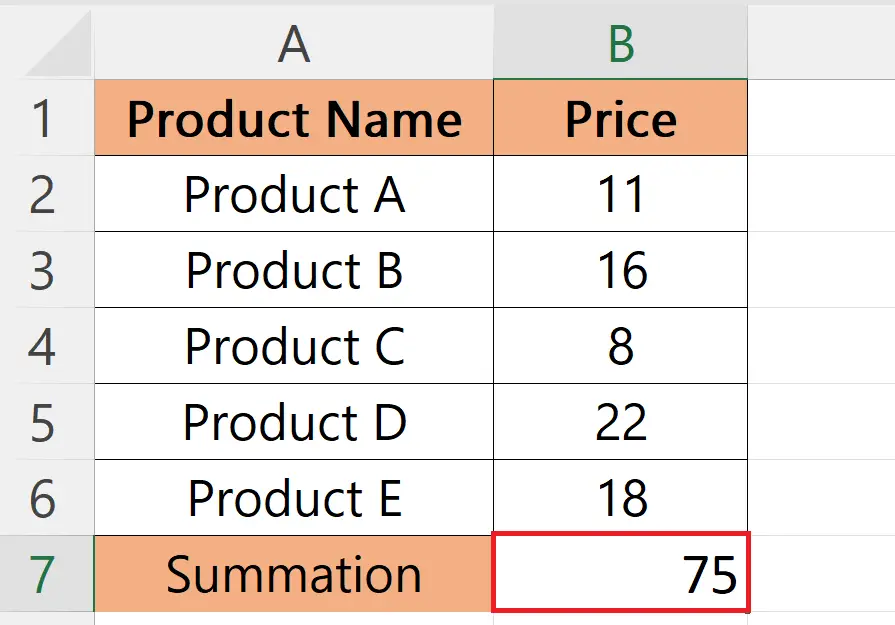
Step 5 – Apply Summation

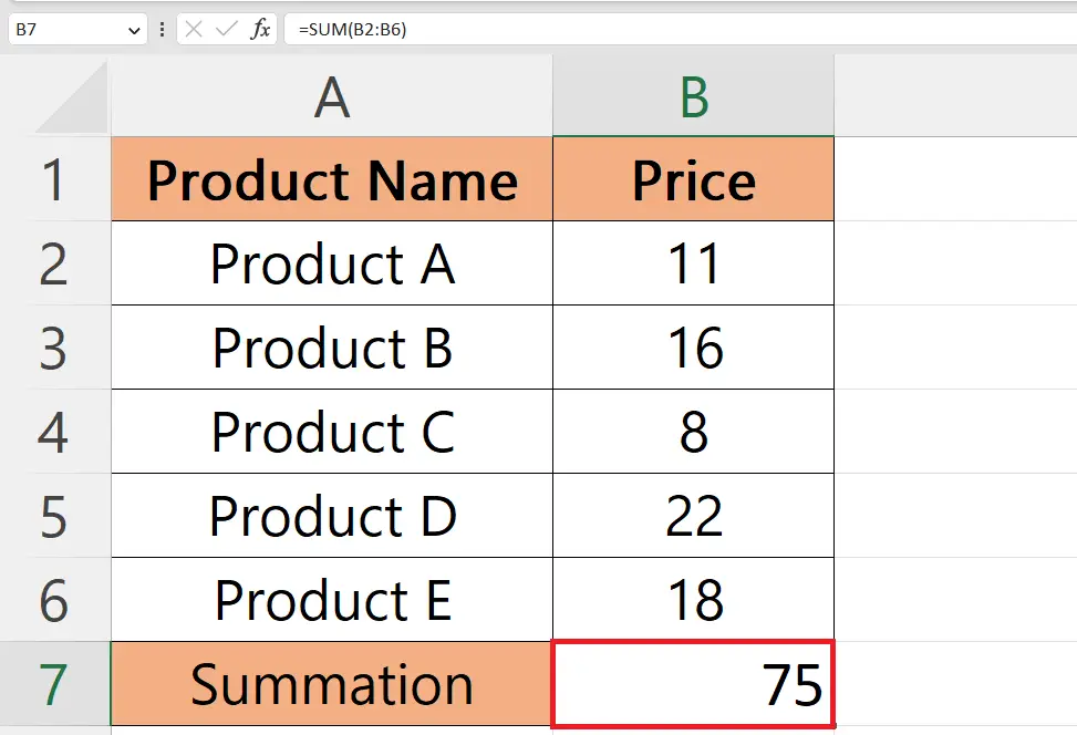
• Apply the summation to the data.

Method 2: Utilizing the “Decrease Decimal” Button

Step 1 – Choose the Cell

• Choose the cell that holds the data you want to round.

Step 2 – Locate the “Decrease Decimal” Button

• Locate the “Decrease Decimal” button in the “Numbers” section of the Home tab.
• Strike the “Decrease Decimal” button the decimal is removed.

Step 3 – Round all the Data

• Follow the above-mentioned steps for all the data.

Step 4 – Apply Summation on the Rounded Data

• Apply summation on the rounded data to get the summation correct.

Method 3: Utilizing the TRUNC Function

Step 1 – Choose an Empty Cell

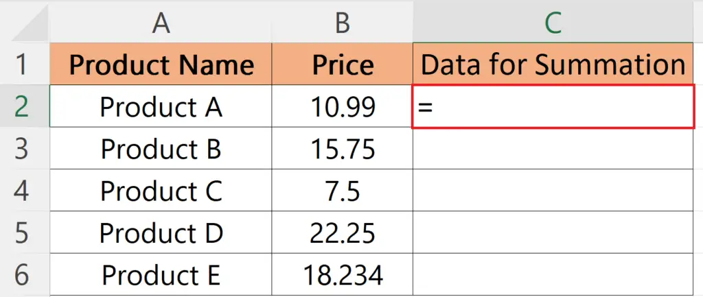
• Choose an Empty cell to apply the TRUNC function.

Step 2 – Enter the TRUNC Function

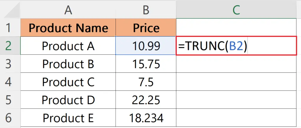
• Enter the TRUNC function:

           TRUNC(B2)

• Where B2 is the cell with the data you want to round.
• Strike the Enter key.

Step 3 – Apply the TRUNC Function on the Complete Data

• Apply the TRUNC function to the complete data utilizing the Autofill feature.

Step 4 – Apply Summation

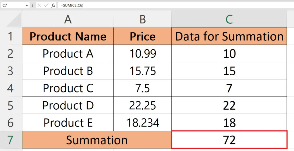
• Apply summation on the data.

Method 4: Utilizing the ROUND Function

Step 1 – Choose an Empty Cell

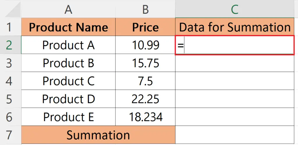
• Choose an Empty cell to apply the TRUNC function.

Step 2 – Enter the ROUND Function

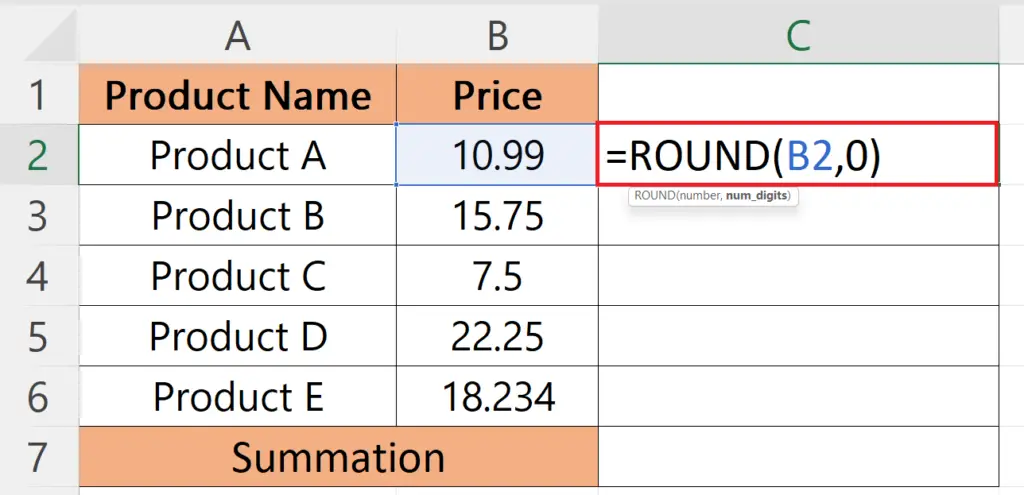
• Enter the ROUND function:

           ROUND(B2,0)

• Where B2 is the cell with the data you want to round and 0 specifies the decimal numbers to be rounded.
• Strike the Enter key.

Step 3 – Apply the ROUND Function on the Complete Data

• Apply the ROUND function to the complete data.

Step 4 – Apply Summation

• Apply summation on the data.