How to rotate contents in Excel

You can watch a video tutorial here.

When formatting a table in Excel, you may need to rotate the contents of a cell to accommodate more columns in the display or to make the table look more appealing.

Option 1 – Use the button on the ribbon

Step 1 – Select the cells

• Select the cells for which the contents are to be rotated

Step 2 – Choose an option for rotation

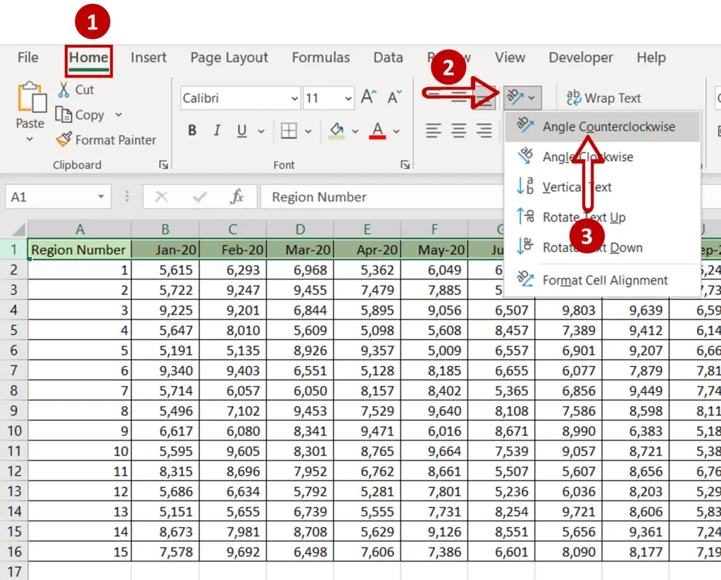
• Go to Home > Alignment
• Expand the Orientation drop-down
• Select Angle Counterclockwise

Step 3 – Check the result

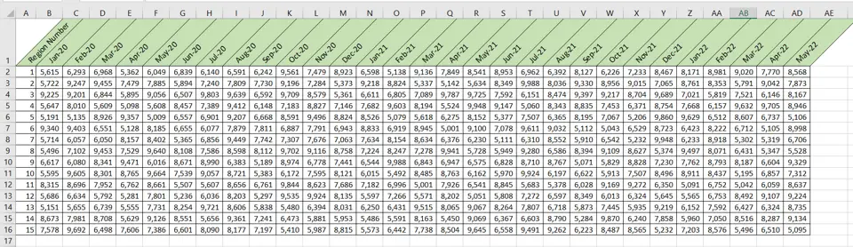
• The text in the cells is rotated to an angle of 45 degrees
• Resize the columns by clicking on the column dividers to accommodate all the columns

Option 2 – Use the Format Cells window

Step 1 – Select the cells

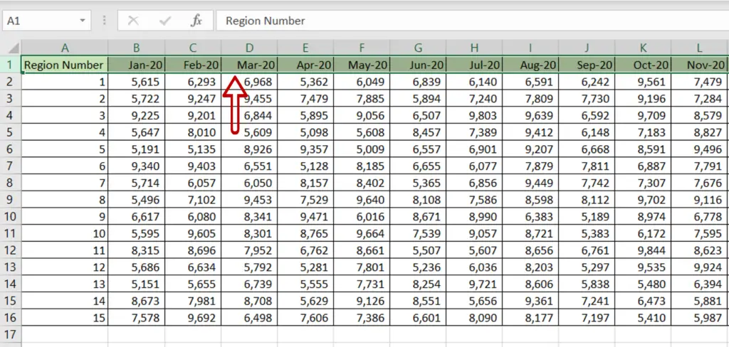
• Select the cells for which the contents are to be rotated

Step 2 – Open the Format Cells window

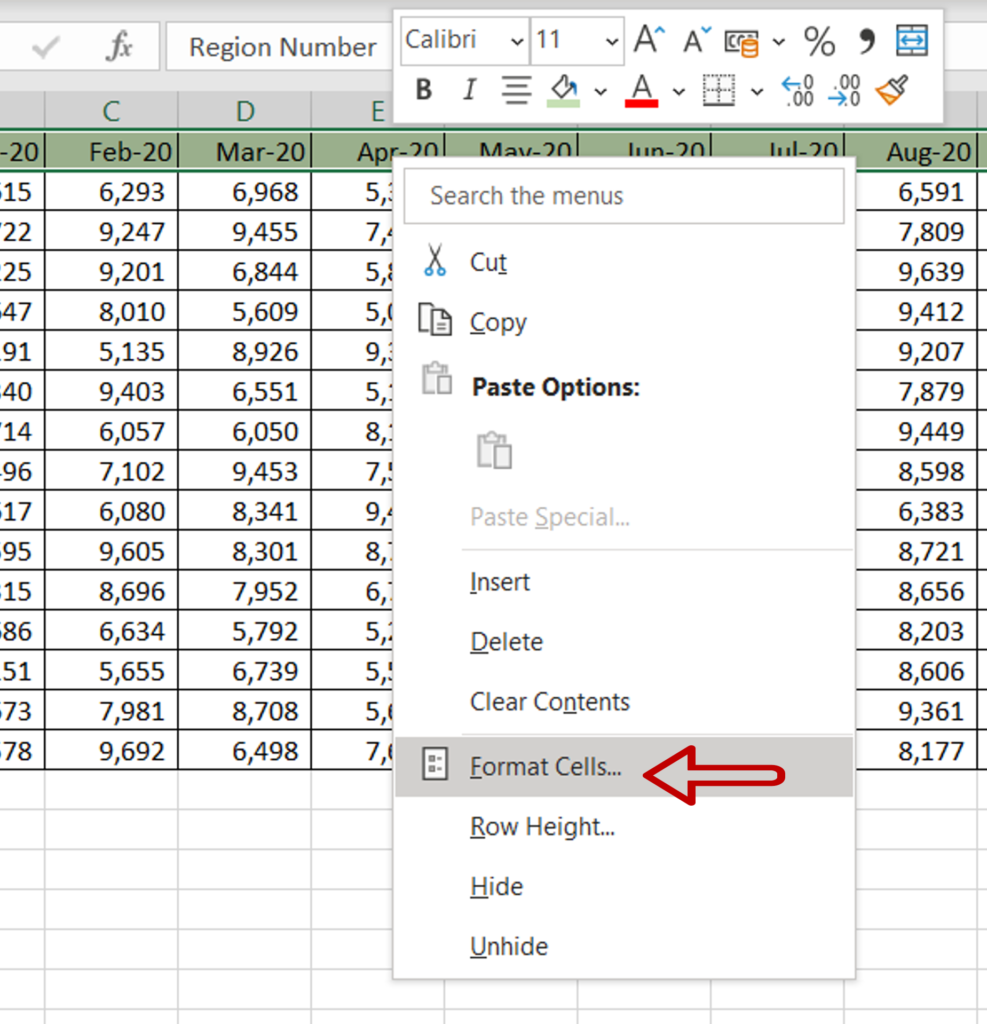
• Right-click and select Format Cells  from the context menu

OR

Go to Home > Number  and click on the arrow to expand the menu

OR

Go to Home > Cells > Format > Format Cells

OR

Press Ctrl+1

Step 3 – Rotate the text

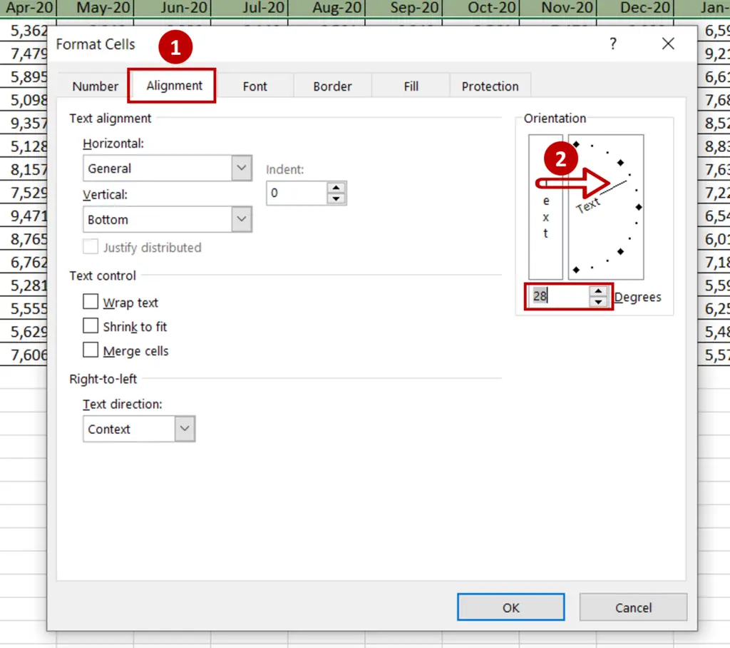
• Go to the Alignment tab
• In the Orientation section, drag the line to rotate the text to 28^o
• The degree of rotation will be displayed below
• Alternatively, type the number of degrees in the box
• Click OK

Step 4 – Check the result

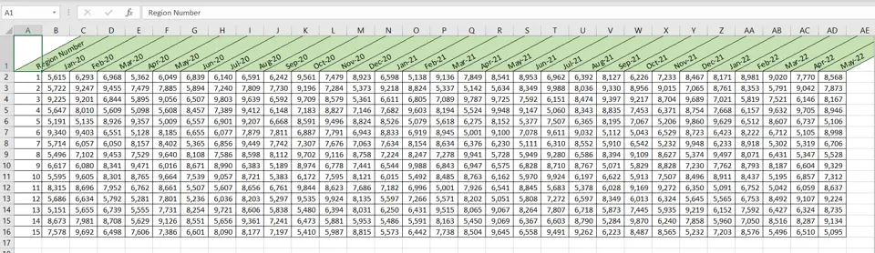
• The text in the cells is rotated to an angle of 28 degrees
• Resize the columns by clicking on the column dividers to accommodate all the columns